AI

基本分类

官网示例：https://www.tensorflow.org/tutorials/keras/basic_classification
主要步骤：

加载Fashion MNIST数据集
探索数据：了解数据集格式
预处理数据
构建模型：设置层、编译模型
训练模型
评估准确率
做出预测：可视化

Fashion MNIST数据集

经典 MNIST 数据集（常用作计算机视觉机器学习程序的“Hello, World”入门数据集）的简易替换
包含训练数据60000个，测试数据10000个，每个图片是28x28像素的灰度图像，涵盖10个类别
https://keras.io/datasets/#fashion-mnist-database-of-fashion-articles
TensorFlow：https://www.tensorflow.org/api_docs/python/tf/keras/datasets/fashion_mnist
GitHub：https://github.com/zalandoresearch/fashion-mnist

tf.keras

Keras是一个用于构建和训练深度学习模型的高级API
TensorFlow中的tf.keras是Keras API规范的TensorFlow实现，可以运行任何与Keras兼容的代码，保留了一些细微的差别
最新版TensorFlow中的tf.keras版本可能与PyPI中的最新Keras版本不同
https://www.tensorflow.org/api_docs/python/tf/keras/

过拟合

如果机器学习模型在新数据上的表现不如在训练数据上的表现，就表示出现过拟合

示例

脚本内容

GitHub：https://github.com/anliven/Hello-AI/blob/master/Google-Learn-and-use-ML/1_basic_classification.py

  1 # coding=utf-8
  2 import tensorflow as tf
  3 from tensorflow import keras
  4 import numpy as np
  5 import matplotlib.pyplot as plt
  6 import os
  7 
  8 os.environ['TF_CPP_MIN_LOG_LEVEL'] = '2'
  9 print("TensorFlow version: {}  - tf.keras version: {}".format(tf.VERSION, tf.keras.__version__))  # 查看版本
 10 
 11 # ### 加载数据集
 12 # 网络畅通的情况下，可以从 TensorFlow 直接访问 Fashion MNIST，只需导入和加载数据即可
 13 # 或者手工下载文件，并存放在“~/.keras/datasets”下的fashion-mnist目录
 14 fashion_mnist = keras.datasets.fashion_mnist
 15 (train_images, train_labels), (test_images, test_labels) = fashion_mnist.load_data()
 16 # 训练集：train_images 和 train_labels 数组，用于学习的数据
 17 # 测试集：test_images 和 test_labels 数组，用于测试模型
 18 # 图像images为28x28的NumPy数组，像素值介于0到255之间
 19 # 标签labels是整数数组，介于0到9之间，对应于图像代表的服饰所属的类别，每张图像都映射到一个标签
 20 
 21 class_names = ['T-shirt/top', 'Trouser', 'Pullover', 'Dress', 'Coat',
 22                'Sandal', 'Shirt', 'Sneaker', 'Bag', 'Ankle boot']  # 类别名称
 23 
 24 # ### 探索数据：了解数据格式
 25 print("train_images.shape: {}".format(train_images.shape))  # 训练集中有60000张图像，每张图像都为28x28像素
 26 print("train_labels len: {}".format(len(train_labels)))  # 训练集中有60000个标签
 27 print("train_labels: {}".format(train_labels))  # 每个标签都是一个介于 0 到 9 之间的整数
 28 print("test_images.shape: {}".format(test_images.shape))  # 测试集中有10000张图像，每张图像都为28x28像素
 29 print("test_labels len: {}".format(len(test_labels)))  # 测试集中有10000个标签
 30 print("test_labels: {}".format(test_labels))
 31 
 32 # ### 预处理数据
 33 # 必须先对数据进行预处理，然后再训练网络
 34 plt.figure(num=1)  # 创建图形窗口，参数num是图像编号
 35 plt.imshow(train_images[0])  # 绘制图片
 36 plt.colorbar()  # 渐变色度条
 37 plt.grid(False)  # 显示网格
 38 plt.savefig("./outputs/sample-1-figure-1.png", dpi=200, format='png')  # 保存文件，必须在plt.show()前使用，否则将是空白内容
 39 plt.show()  # 显示
 40 plt.close()  # 关闭figure实例，如果要创建多个figure实例，必须显示调用close方法来释放不再使用的figure实例
 41 
 42 # 值缩小为0到1之间的浮点数
 43 train_images = train_images / 255.0
 44 test_images = test_images / 255.0
 45 
 46 # 显示训练集中的前25张图像，并在每张图像下显示类别名称
 47 plt.figure(num=2, figsize=(10, 10))  # 参数figsize指定宽和高，单位为英寸
 48 for i in range(25):  # 前25张图像
 49     plt.subplot(5, 5, i + 1)
 50     plt.xticks([])  # x坐标轴刻度
 51     plt.yticks([])  # y坐标轴刻度
 52     plt.grid(False)
 53     plt.imshow(train_images[i], cmap=plt.cm.binary)
 54     plt.xlabel(class_names[train_labels[i]])  # x坐标轴名称
 55 plt.savefig("./outputs/sample-1-figure-2.png", dpi=200, format='png')
 56 plt.show()
 57 plt.close()
 58 
 59 # ### 构建模型
 60 # 构建神经网络需要先配置模型的层，然后再编译模型
 61 # 设置层
 62 model = keras.Sequential([
 63     keras.layers.Flatten(input_shape=(28, 28)),  # 将图像格式从二维数组（28x28像素）转换成一维数组（784 像素）
 64     keras.layers.Dense(128, activation=tf.nn.relu),  # 全连接神经层，具有128个节点（或神经元）
 65     keras.layers.Dense(10, activation=tf.nn.softmax)])  # 全连接神经层，具有10个节点的softmax层
 66 # 编译模型
 67 model.compile(optimizer=tf.train.AdamOptimizer(),  # 优化器：根据模型看到的数据及其损失函数更新模型的方式
 68               loss='sparse_categorical_crossentropy',  # 损失函数：衡量模型在训练期间的准确率。
 69               metrics=['accuracy'])  # 指标：用于监控训练和测试步骤；这里使用准确率（图像被正确分类的比例）
 70 
 71 # ### 训练模型
 72 # 将训练数据馈送到模型中，模型学习将图像与标签相关联
 73 model.fit(train_images,  # 训练数据
 74           train_labels,  # 训练数据
 75           epochs=5,  # 训练周期（训练模型迭代轮次）
 76           verbose=2  # 日志显示模式：0为安静模式, 1为进度条（默认）, 2为每轮一行
 77           )  # 调用model.fit 方法开始训练，使模型与训练数据“拟合
 78 
 79 # ### 评估准确率
 80 # 比较模型在测试数据集上的表现
 81 test_loss, test_acc = model.evaluate(test_images, test_labels)
 82 print('Test loss: {} - Test accuracy: {}'.format(test_loss, test_acc))
 83 
 84 # ### 做出预测
 85 predictions = model.predict(test_images)  # 使用predict()方法进行预测
 86 print("The first prediction: {}".format(predictions[0]))  # 查看第一个预测结果(包含10个数字的数组，分别对应10种服饰的“置信度”
 87 label_number = np.argmax(predictions[0])  # 置信度值最大的标签
 88 print("label: {} - class name: {}".format(label_number, class_names[label_number]))
 89 print("Result true or false: {}".format(test_labels[0] == label_number))  # 对比测试标签，查看该预测是否正确
 90 
 91 
 92 # 可视化：将该预测绘制成图来查看全部10个通道
 93 def plot_image(m, predictions_array, true_label, img):
 94     predictions_array, true_label, img = predictions_array[m], true_label[m], img[m]
 95     plt.grid(False)
 96     plt.xticks([])
 97     plt.yticks([])
 98     plt.imshow(img, cmap=plt.cm.binary)
 99     predicted_label = np.argmax(predictions_array)
100     if predicted_label == true_label:
101         color = 'blue'  # 正确的预测标签为蓝色
102     else:
103         color = 'red'  # 错误的预测标签为红色
104     plt.xlabel("{} {:2.0f}% ({})".format(class_names[predicted_label],
105                                          100 * np.max(predictions_array),
106                                          class_names[true_label]),
107                color=color)
108 
109 
110 def plot_value_array(n, predictions_array, true_label):
111     predictions_array, true_label = predictions_array[n], true_label[n]
112     plt.grid(False)
113     plt.xticks([])
114     plt.yticks([])
115     thisplot = plt.bar(range(10), predictions_array, color="#777777")
116     plt.ylim([0, 1])
117     predicted_label = np.argmax(predictions_array)
118     thisplot[predicted_label].set_color('red')
119     thisplot[true_label].set_color('blue')
120 
121 
122 # 查看第0张图像、预测和预测数组
123 i = 0
124 plt.figure(num=3, figsize=(8, 5))
125 plt.subplot(1, 2, 1)
126 plot_image(i, predictions, test_labels, test_images)
127 plt.subplot(1, 2, 2)
128 plot_value_array(i, predictions, test_labels)
129 plt.xticks(range(10), class_names, rotation=45)  # x坐标轴刻度，参数rotation表示label旋转显示角度
130 plt.savefig("./outputs/sample-1-figure-3.png", dpi=200, format='png')
131 plt.show()
132 plt.close()
133 
134 # 查看第12张图像、预测和预测数组
135 i = 12
136 plt.figure(num=4, figsize=(8, 5))
137 plt.subplot(1, 2, 1)
138 plot_image(i, predictions, test_labels, test_images)
139 plt.subplot(1, 2, 2)
140 plot_value_array(i, predictions, test_labels)
141 plt.xticks(range(10), class_names, rotation=45)  # range(10)作为x轴的刻度，class_names作为对应的标签
142 plt.savefig("./outputs/sample-1-figure-4.png", dpi=200, format='png')
143 plt.show()
144 plt.close()
145 
146 # 绘制图像：正确的预测标签为蓝色，错误的预测标签为红色，数字表示预测标签的百分比（总计为 100）
147 num_rows = 5
148 num_cols = 3
149 num_images = num_rows * num_cols
150 plt.figure(num=5, figsize=(2 * 2 * num_cols, 2 * num_rows))
151 for i in range(num_images):
152     plt.subplot(num_rows, 2 * num_cols, 2 * i + 1)
153     plot_image(i, predictions, test_labels, test_images)
154     plt.subplot(num_rows, 2 * num_cols, 2 * i + 2)
155     plot_value_array(i, predictions, test_labels)
156     plt.xticks(range(10), class_names, rotation=45)
157 plt.savefig("./outputs/sample-1-figure-5.png", dpi=200, format='png')
158 plt.show()
159 plt.close()
160 
161 # 使用经过训练的模型对单个图像进行预测
162 image = test_images[0]  # 从测试数据集获得一个图像
163 print("img shape: {}".format(image.shape))  # 图像的shape信息
164 image = (np.expand_dims(image, 0))  # 添加到列表中
165 print("img shape: {}".format(image.shape))
166 predictions_single = model.predict(image)  # model.predict返回一组列表，每个列表对应批次数据中的每张图像
167 print("prediction_single: {}".format(predictions_single))  # 查看预测，预测结果是一个具有10个数字的数组，分别对应10种不同服饰的“置信度”
168 
169 plt.figure(num=6)
170 plot_value_array(0, predictions_single, test_labels)
171 plt.xticks(range(10), class_names, rotation=45)
172 plt.savefig("./outputs/sample-1-figure-6.png", dpi=200, format='png')
173 plt.show()
174 plt.close()
175 
176 prediction_result = np.argmax(predictions_single[0])  # 获取批次数据中相应图像的预测结果（置信度值最大的标签）
177 print("prediction_result: {}".format(prediction_result))

运行结果

common line

C:UsersanlivenAppDataLocalcondacondaenvsmlccpython.exe D:/Anliven/Anliven-Code/PycharmProjects/TempTest/TempTest.py
TensorFlow version: 1.12.0
train_images.shape: (60000, 28, 28)
train_labels len: 60000
train_labels: [9 0 0 ... 3 0 5]
test_images.shape: (10000, 28, 28)
test_labels len: 10000
test_labels: [9 2 1 ... 8 1 5]
Epoch 1/5
 - 3s - loss: 0.5077 - acc: 0.8211
Epoch 2/5
 - 3s - loss: 0.3790 - acc: 0.8632
Epoch 3/5
 - 3s - loss: 0.3377 - acc: 0.8755
Epoch 4/5
 - 3s - loss: 0.3120 - acc: 0.8855
Epoch 5/5
 - 3s - loss: 0.2953 - acc: 0.8914

   32/10000 [..............................] - ETA: 15s
 2208/10000 [=====>........................] - ETA: 0s 
 4576/10000 [============>.................] - ETA: 0s
 7008/10000 [====================>.........] - ETA: 0s
 9344/10000 [===========================>..] - ETA: 0s
10000/10000 [==============================] - 0s 30us/step
Test loss: 0.3584352566242218 - Test accuracy: 0.8711
The first prediction: [4.9706377e-06 2.2675355e-09 1.3649772e-07 3.6149192e-08 4.7982059e-08
 8.5262489e-03 1.5245891e-05 3.2628113e-03 1.6874857e-05 9.8817366e-01]
label: 9 - class name: Ankle boot
Result true or false: True
img shape: (28, 28)
img shape: (1, 28, 28)
prediction_single: [[4.9706327e-06 2.2675313e-09 1.3649785e-07 3.6149192e-08 4.7982059e-08
  8.5262526e-03 1.5245891e-05 3.2628146e-03 1.6874827e-05 9.8817366e-01]]
prediction_result: 9

Process finished with exit code 0

Figure1

Figure2

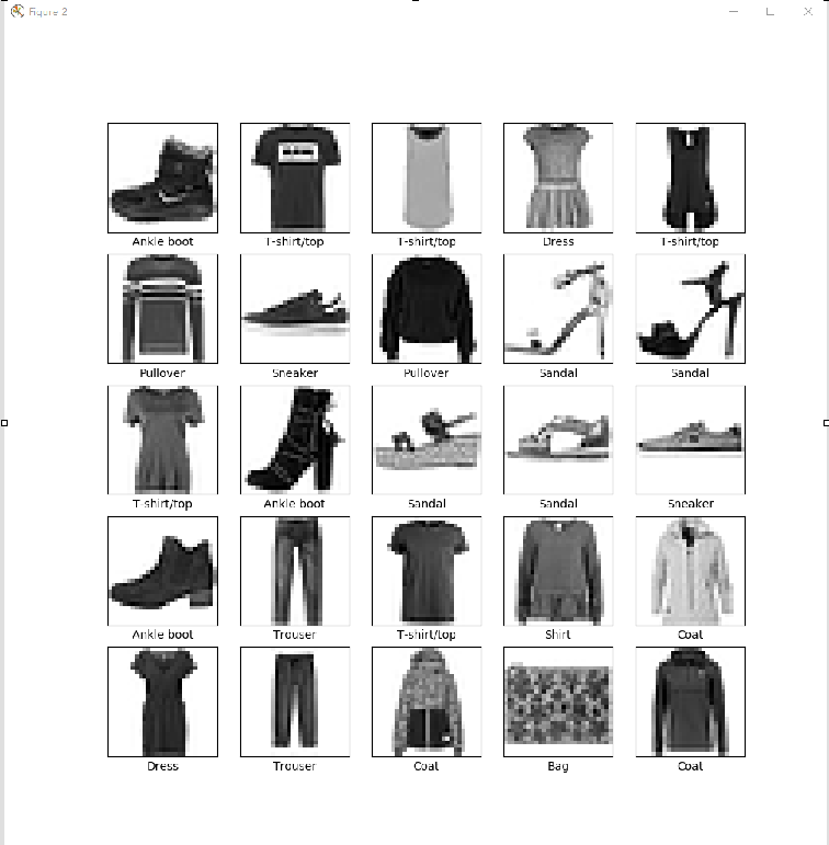
Figure3

Figure4

Figure5

Figure6

问题处理

问题1：执行fashion_mnist.load_data()失败

错误提示
Downloading data from https://storage.googleapis.com/tensorflow/tf-keras-datasets/train-labels-idx1-ubyte.gz
......
Exception: URL fetch failure on https://storage.googleapis.com/tensorflow/tf-keras-datasets/train-labels-idx1-ubyte.gz: None -- [WinError 10060] A connection attempt failed because the connected party did not properly respond after a period of time, or established connection failed because connected host has failed to respond

处理方法1

选择一个链接，

手工下载下面四个文件，并存放在“~/.keras/datasets”下的fashion-mnist目录。

train-labels-idx1-ubyte.gz
train-images-idx3-ubyte.gz
t10k-labels-idx1-ubyte.gz
t10k-images-idx3-ubyte.gz

guowli@5CG450158J MINGW64 ~/.keras/datasets
$ pwd
/c/Users/guowli/.keras/datasets

guowli@5CG450158J MINGW64 ~/.keras/datasets
$ ls -l
total 0
drwxr-xr-x 1 guowli 1049089 0 Mar 27 14:44 fashion-mnist/

guowli@5CG450158J MINGW64 ~/.keras/datasets
$ ls -l fashion-mnist/
total 30164
-rw-r--r-- 1 guowli 1049089  4422102 Mar 27 15:47 t10k-images-idx3-ubyte.gz
-rw-r--r-- 1 guowli 1049089     5148 Mar 27 15:47 t10k-labels-idx1-ubyte.gz
-rw-r--r-- 1 guowli 1049089 26421880 Mar 27 15:47 train-images-idx3-ubyte.gz
-rw-r--r-- 1 guowli 1049089    29515 Mar 27 15:47 train-labels-idx1-ubyte.gz

处理方法2

手工下载文件，存放在指定目录。
改写“tensorflowpythonkerasdatasetsfashion_mnist.py”定义的load_data()函数。

from tensorflow.python.keras.utils import get_file
import numpy as np
import pathlib
import gzip


def load_data():  # 改写“tensorflowpythonkerasdatasetsfashion_mnist.py”定义的load_data()函数
    base = "file:///" + str(pathlib.Path.cwd()) + "\"  # 当前目录

    files = [
        'train-labels-idx1-ubyte.gz', 'train-images-idx3-ubyte.gz',
        't10k-labels-idx1-ubyte.gz', 't10k-images-idx3-ubyte.gz'
    ]

    paths = []
    for fname in files:
        paths.append(get_file(fname, origin=base + fname))

    with gzip.open(paths[0], 'rb') as lbpath:
        y_train = np.frombuffer(lbpath.read(), np.uint8, offset=8)

    with gzip.open(paths[1], 'rb') as imgpath:
        x_train = np.frombuffer(
            imgpath.read(), np.uint8, offset=16).reshape(len(y_train), 28, 28)

    with gzip.open(paths[2], 'rb') as lbpath:
        y_test = np.frombuffer(lbpath.read(), np.uint8, offset=8)

    with gzip.open(paths[3], 'rb') as imgpath:
        x_test = np.frombuffer(
            imgpath.read(), np.uint8, offset=16).reshape(len(y_test), 28, 28)

    return (x_train, y_train), (x_test, y_test)


(train_images, train_labels), (test_images, test_labels) = load_data()

问题2：使用gzip.open()打开.gz文件失败

错误提示

“OSError: Not a gzipped file (b' ')”

处理方法

对于损坏的、不完整的.gz文件，zip.open()将无法打开。检查.gz文件是否完整无损。

参考信息

https://github.com/tensorflow/tensorflow/issues/170