承接上一章,接着写Genetic Algorithm。
本章主要写排列表达(permutation representations)
开始先引一个具体的例子来进行表述
Outline
- 问题描述
- 排列表达的变异算子
- 排列表达的重组算子
- 种群模型
- 父辈选择
1. 问题描述
旅行商问题。给定n个城市,旅行商需要拜访所有城市后回到原点。要求每个城市只能拜访一次,问题的最终目标是寻找一个最短的路线。

Encoding: 将所有的城市标上序号:1,2,...,n。比如n=4,那么排列可以为[1,2,3,4]或者[3,4,2,1]
现在问题给定有30个城市,那么一共有30!种不同的路线,30!≈10^32
A non polynomial algorithm, where the computational effort taken is not described as a polynomial function of the problem size.
2. 排列表达的变异算子(mutation operators for permutations)
在这个问题中,常规的变异算子会导致一些无法执行的方案(inadmissible solutions)。比如说,将某一位上的值j变异为了k,那么就会导致去了两次城市k,而一次都没有去城市j。所以每次变异,必须同时变掉两个。
2.1 插入式变异(Insert mutation for permutations)
随机找两个等位基因。讲第二个基因移动到紧接着第一个基因的位置,其他位置的基因顺着移动一个位置。
![]()
特点:保存了大多数基因的顺序信息和相邻信息。
Note this preserves most of the order and the adjacency information
2.2 交换式变异(swap mutation for permutations)
随机找两个等位基因,交换他们的位置。
![]()
特点:保存了大多数的相邻信息,但是扰乱了顺序
Preserves most of adjacency information (4 links broken), disrupts order more
2.3 倒置式变异(inversion mutation for permutations)
随机选择两个等位基因,然后将位于这两个等位基因之间的子序列倒置。
![]()
特点:保存了大多数的相邻信息,但是造成了顺序上的破坏。
preserves most adjacency information(only breaks two links) but disruptive of order information
2.4 混乱式变异(scramble mutation for permutations)
选取基因的一个子序列,随机地进行重新排列。
![]()
注意这个子序列并不一定要求是连续的。
3. 排列表达的重组算子(crossover operators for permutations)
和变异算子一样,在这个问题中常规的重组算子也有可能造成题目的无解(inadmissible solutions)。
比如下面这种情况:

这里提出的所有算子,都会专注于父辈的顺序信息和相邻信息这两方面的保存。
3.1 地图式重组 partially mapped crossover (PMX)
首先,在第一个父辈(P1)里随机选择两个重组的点(crossover points),把这两个点之间的基因拿出来,放到第一个后代的相应位置上去。
接着,从上述的第一个重组的点开始,寻找第二个父辈(P2)在相应位置上还没有被copy的基因。比如说这里的第一个数字是P2中的8,对应于P1相应位置的是4,而4在P2里的位置在最后一个点,因此把8放到后代的最后一个点。第二个数字是P2中的2,对应于P1相应位置的是5,而5已经被copy到了第一个后代上去了,所以我们寻找与P2上5的位置相对应的 P1位置上的数字是7,接着看到7在P2上的位置是第三个,因此把2放到了第三个位置上。
第三个数字是6,第四个数字是5,然而这两个数字已经同时存在于两个父辈的copy基因段上。
最后一步是copy剩余的元素到后代的相同位置上。

第二个后代的产生和第一个类似,但是将两个父辈的角色位置对调。
Informal procedure for parents P1 and P2:
- Choose random segment and copy it from P1
- Starting from the first crossover point look for elements in that segment of P2 that have not been copied
- For each of these i look in the offspring to see what element j has been copied in its place from P1
- Place i into the position occupied j in P2, since we know that we will not be putting j there (as is already in offspring)
- If the place occupied by j in P2 has already been filled in the offspring k, put i in the position occupied by k in P2
- Having dealt with the elements from the crossover segment, the rest of the offspring can be filled from P2. Second child is created analogously
3.2 顺序重组(order crossover)
顺序重组算子(order crossover operator)是用来对付以顺序为基础的序列问题。
首先从第一个父辈那里随机地选择两个重组点,将他们之间的片段copy到第一个后代的对应位置上面去。
接着,从第二个重组点的位置开始,在第二个父辈的相应位置copy剩余的基因,第一个copy的是数字1,第二个数字4由于已经copy过了,所以跳过它,接着后面是9,3,8,2。遇到末尾时候自动跳转到头部位置。

第二个后代的产生和第一个类似,但是将两个父辈的角色位置对调。
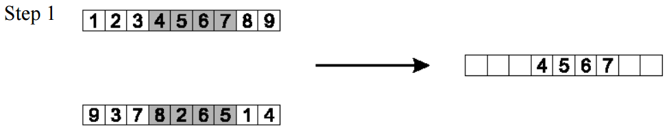
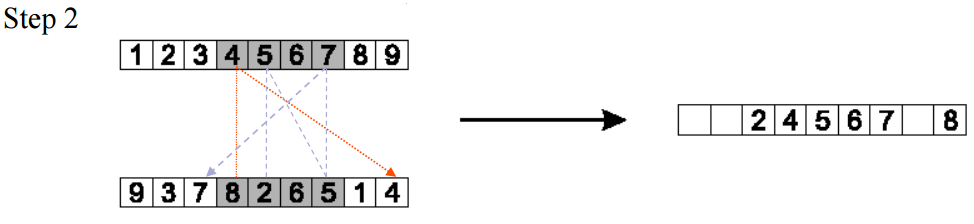
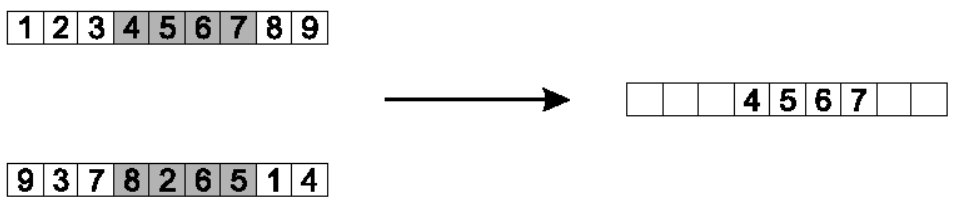
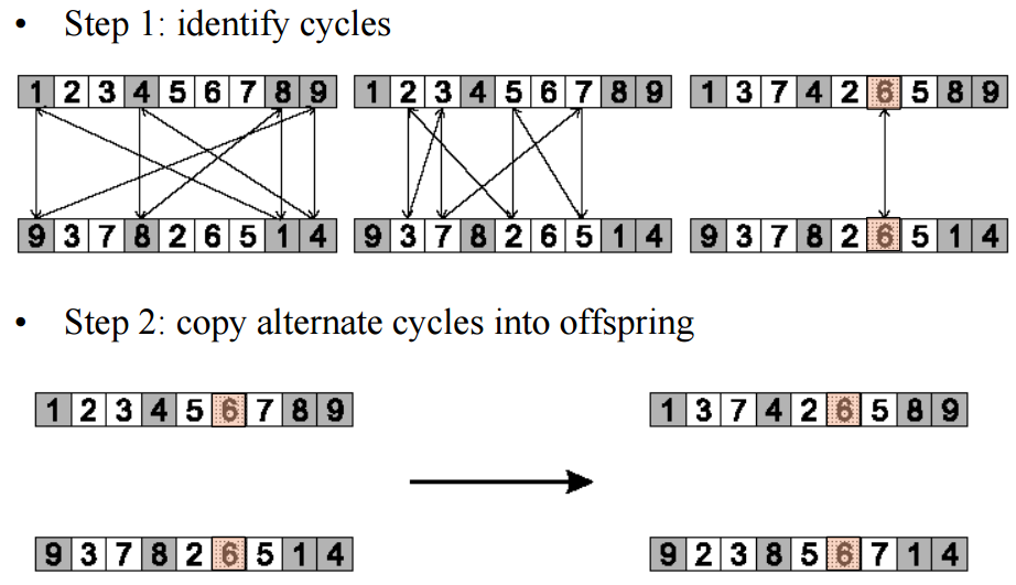
3.3 循环重组(cycle crossover)
基本思想:每一个从父辈那里获取的等位基因,是伴随着他原来的位置的。
Informal procedure:
1. Make a cycle of alleles from P1 in the following way:
(a) start with the first allele of P1.
(b) look at the allele at the same position in P2.
(c) go to the position with the same allele in P1.
(d) add this allele to the cycle.
(e) repeat step b through d until you arrive at the first allele of P1.
2. Put the alleles of the cycle in the first child on the positions they have in the first parent.
3. Take next cycle from second parent.
下图展示的数据还是接着TSP的例子来说的。
3.4 边重组(edge crossover)
Edge crossover is based on the idea that an offspring should be created as far as possible using only edges that are present in one or more parent.
接着TSP的例子来说,比如现在有两个父辈,有两条路线,分别是[1 2 3 4 5 6 7 8 9]和[9 3 7 8 2 6 5 1 4]。首先构建一张表格,写出每一个城市以及和他相邻的城市(无论在P1还是P2中)。用"+"来表示这个城市同时在P1和P2中与目标城市相邻。

接下来是边重组(edge crossover)的过程:
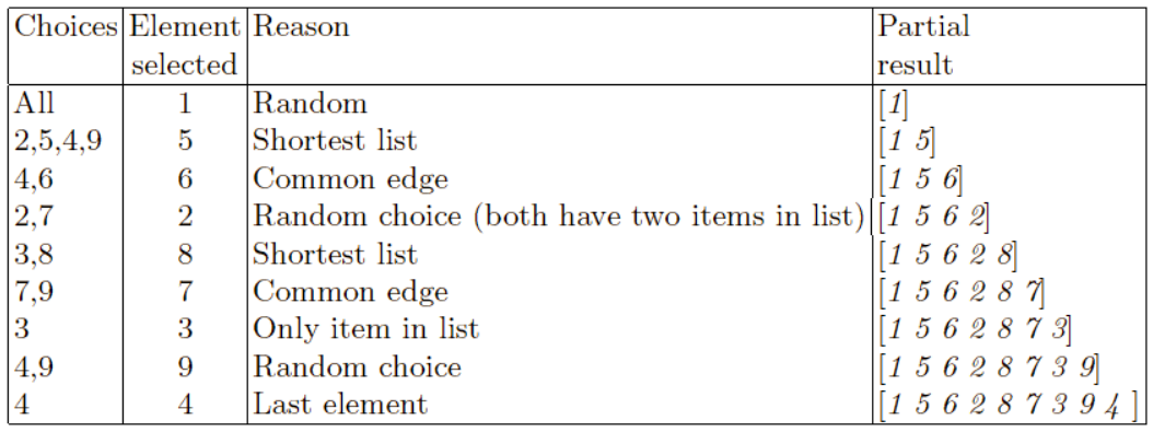
这个过程的文字性描述如下:
In formal procedure once edge once table is constructed:
1. Pick an initial element at random and put it in the offspring.
2. Set the variable current element = entry
3. Remove all references to current element from the table
4. Example list for current element:
-
-
- If there is a common edge, pick that to be next element.
- Otherwise pick the entry in the list which itself has the shortest list
- Ties are split at random
-
5. In the case of reaching an empty list:
-
-
- Examine the other end of the offspring is for extension
- Otherwise a new element is chosen at random
-
3.5 多父辈的重组(multiparent recombination)
自然界的进化遗传中,通常是由两个父辈结合产生后代的。考虑到我们的算法并不受自然实际规律的约束,也可能存在多父辈结合的情况。
不能说增加重组的参数数量就“一定”是有利的,要具体问题具体地对待。不过,已经有大量的试验表明,使用超过两个父辈往往是有利的。
变异需要1个父辈,重组需要2个父辈。这里的多父辈遗传会超过2个父辈。
本系列博客不过多讲述多父辈的情况,仅摘录原文如下:
Three main types:
- Based on allele frequencies, e.g., p-sexual voting generalising uniform crossover
- Based on segmentation and recombination of the parents, e.g., diagonal crossover generalising n-point crossover
- Based on numerical operations on real-valued alleles, e.g., center of mass crossover, generalising arithmetic recombination operators
4. 种群模型(population models)
4.1 一代模型(generational model)
SGA(simple genetic algorithm)就是使用了“一代模型”(generational model):
- 每一个个体仅仅存活一代
- 整个父代一代会被后代全部替代掉
引述原文如下:
In each generation we begin with a population of size μ, from which a mating pool of μ parents is selected. Next, λ(=μ) offspring are created from the mating pool by the application of variation operators, and evaluated. After each generation, the whole population is replaced by its offspring, which is called the "next generation".
4.2 稳定状态模型(steady-state model)
- 每一代只产生一个后代
- 产生后种群中的一个成员会被替换掉
引述原文如下:
In the steady-state model, the entire population is not changed at once, but rather a part of it. In this case, λ(<μ) old individuals are replaced by λ new ones, the offspring. The percentage of the population that is replaced is called the generational gap, and is equal to λ/μ。
The steady-state model has been widely studied and applied, usually with λ=1 and a corresponding generation gap of 1/μ。
5. 父代选择(parent selection)
下面的几种选择方式,是用来确定一个概率的分布,这个概率的分布是用来决定种群中每一个个体(mating pool中的个体)被选择进行繁殖的概率。
5.1 适应-比例选择(fitness-proportionate selection, FPS)
在上一章"简单基因算法"(SGA)的例子f(x) = x^2中有提到,这种选择的概率是:
![]()
分子上是个体,分母上是整个种群。
这种选择会面临的一些缺点:
- 过早的收敛(premature convergence) :一些杰出的个体会过早地占领整个种群。
- 当种群中的个体都非常接近的时候,会导致缺乏选择的压力(no selection pressure)。当开始收敛,并且坏的个体被淘汰掉的时候,这个种群的进化将会非常的缓慢。
- Highly susceptible to function transposition: The mechanism behaves differently on transposed versions of the same fitness function.原方程稍微变一下,就会对这个机制造成很大影响。
下面有一个例子,来说明上述缺点的最后一点。从第二张饼状图中可以看出,如果仅仅用“适应-比例选择”(FPS)方法的话,在A、B、C三点上,每个点所占比例发生了变化。

It shows the changes in selection probabilities for three points that arise when a random fitness function y = f(x) is transposed by adding 10.0 to all fitness values. As can be seen the selective advantage of the fittest point (B) is reduced.
为了弥补上述的第二个和第三个缺点,这里介绍两种方法:
- Windowing:在这个方法中,通过减去一个f(x)中的值,适应度之间的差别将会被保留。最简单的方式就是减去种群中适应度最差的那个值。另一个选择是减去最后几代种群中的平均值。β is worst fitness in this (last n) generations.
![]()
- Sigma scaling:另一个非常著名的方法是Goldberg's提出的sigma scaling
f’(i) = max( f(i) – (〈 f 〉 - c • σf ), 0.0)
where c is a constant, usually 2.0
5.2 排序选择(ranking selection)
排序选择(ranking selection)可以弥补 适应-比例选择(fitness-proportionate selection, FPS)的一些缺陷。
依据适应度,ranking selection对种群中的个体进行排序,接着根据这个排序来决定这些个体被选择的概率。这里和适应-比例选择(FPS)的区别在于,FPS是根据这些个体的适应度多少来决定被选择的概率的(selection probabilities),而ranking selection则是根据刚刚的排序来决定被选择的概率的,这样可以保持一个连续性的选择压力(a constant selection pressure)。从rank number到选择概率的转变是很随意的,它可以通过几种不同的方式进行,比如线性地或者以指数方式地减少,当然整个总群的选择概率之和是一定保持不变的。
下面是概率的公式:
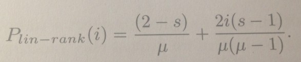
公式中有一个参数s,通常取值在(1.0,2.0]之间。在GA(gennetic algorithm)问题中通常μ = λ。参数i表示rank的值。
下面是一个具体的例子:

这个例子展示了FPS和LRS,以及在s取不同值情况下的LRS。(fitness-proportionate selection,linear ranking selection)
除了上面的linear ranking scheme,再介绍一种exponential ranking scheme
When a linear mapping is used from rank to selection probabilities, the amount of selection pressure that can be applied is limited. This arises from the assumption that, on average, an individual of median fitness should have one chance to be reproduced, which in turn imposes a maximum value of s = 2.0. If a higher selection pressure is required, ie, more emphasis on selecting individuals of above-average fitness, an exponential ranking scheme is often used, of the form:
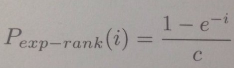
The normalisation factor c is chosen so that the sum of the probabilities is unity, ie, it is a function of the population size.
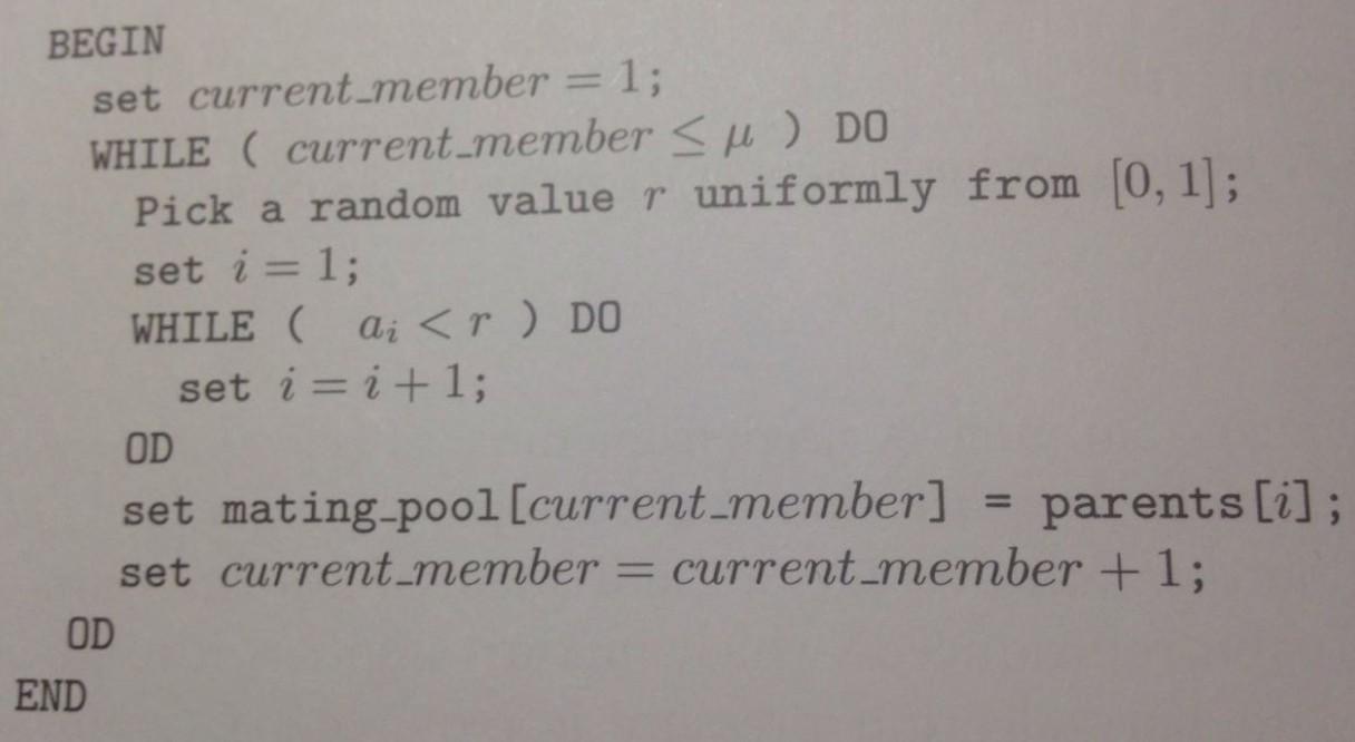
5.3 轮盘赌选择法(roulette wheel)
一个最简单的取样方式是轮盘赌(roulette wheel)。对轮盘赌的详尽描述可见:http://www.cnblogs.com/adelaide/articles/5679475.html
下图是轮盘赌伪代码
Assuming some order over the population(ranking or random) from 1 to μ, we calculate a list of values [a1,a2,....,aμ] such that ![]() ,where
,where ![]() is defined by the selection distribution —— fitness proportionate or ranking.
is defined by the selection distribution —— fitness proportionate or ranking.
5.4 随机遍历取样法(stochastic universal sampling algorithm, SUS)
除了轮盘赌(roulette wheel),另一个放假叫做随机遍历取样(stochastic universal sampling algorithm)
下图是轮盘赌伪代码

占位
5.5 锦标赛选择法(tournament selection)
伪代码如下:
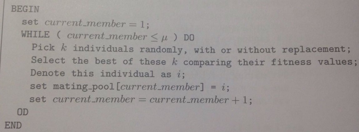
锦标赛选择法(tournament selection)适用于以下情况:
- the population size is very large
- The population is distributed in some way(perhaps on a parallel system), obtaining this knowledge is either highly time consuming or at worst impossible.
锦标赛选择法(tournament selection)具有以下特点:
- does not require any global knowledge of the population
- relies on an ordering relation that can rank any two individuals
- conceptually simple and fast to implement and apply
个体被选择的依据:
- 在种群中的排序。Its rank in the population: effectively this is estimated without the need for sorting the whole population.
- 锦标赛的大小。The tournament size. The larger the tournament, the more chance that it will contain members of above-average fitness, and the less that it will consist entirely of low-fitness members.
- The probability p that the most fit member of the tournament is selected. Usually this is 1.0 (deterministic tournaments), but stochastic versions are also used with p<1.0. Clearly in this case there is lower selection pressure.
- Whether individuals are chosen with or without replacement. In the second case, with deterministic tournaments, the k-1 least-fit members of the population can never be selected, whereas if the tournament candidates are picked with replacement, it is always possible for even the least-fit member of the population to be selected as a result of a lucky draw.
在所有选择方法中,锦标赛选择法是GA算法中被运用得最广泛的算法。due to its simplicity and the fact that the selection pressure is easy to control by varying the tournament size K.