1 Introduction and Motivation
For a given accuracy level, it is typically possible to identify multiple CNN architectures that achieve that accuracy level.
Advantages of smaller CNN architectures:
More efficient distributed training. Communication overhead is directly proportional to the number of parameters in the model for distributed data-parallel training
Less overhead when exporting new models to clients. Smaller models require less communication, making frequent updates more feasible.
Feasible FPGA and embedded deployment. A sufficiently small model could be stored directly on-chip
SqueezeNet achieves AlexNet-level accuracy on ImageNet with 50x fewer parameters and can be compressed to less than 0.5MB(510x smaller than AlexNet)
2 Related Work
2.1 Model Compression
Overarching(首要的) Goal:Identify a model that has very few parameters while preserving accuracy.
A sensible thought:Take an existing CNN model and compress it in a lossy fashion.
Several approaches:
SVD:Apply singular value decomposition(SVD)to a pretrained CNN model(Denton et al., 2014).
Network Pruning: Begin with a pretrained model,replace parameters that are below a certain threshold with zeros to form a sparse matrix,and finally performs a few iterations of training on the sparse CNN(Hanetal.,2015b).
Deep Compression:Combine Network Pruning with quantization (to 8 bits or less) and huffman encoding to create a new approach (Han et al., 2015a), and further designed a hardware accelerator called EIE(Hanetal.,2016a)that operates directly on the compressed model,achieving substantial speedups and energy savings.
2.2 CNN Microarchitecture
In neural networks, convolution filters are typically 3D, with height, width, and channels as the key dimensions. In each subsequent layer Li the filters have the same number of channels as Li-1 has filters.
With the trend of designing very deep CNNs, it becomes cumbersome to manually select filter dimensions for each layer. To address this,various higher level building blocks,or modules,comprised of multiple convolution layers with a specific fixed organization have been proposed.
Example:GoogLeNet Inception modules including 1x1 and 3x3, plus sometimes 5x5 (Szegedy et al., 2014) and sometimes 1x3 and 3x1.
Many such modules are then combined,perhaps with additional ad-hoc layers, to form a complete network.
We use the term(术语) CNN microarchitecture to refer to the particular organization and dimensions of the individual modules.
2.3 CNN Macroarchitecture
While the CNN microarchitecture refers to individual layers and modules, we define the CNN macroarchitecture as the system-level organization of multiple modules into an end-to-end CNN architecture.
Perhaps the mostly widely studied CNN macroarchitecture topicintherecentliteratureistheimpact ofdepth(i.e. numberoflayers)innetworks.
The choice of connections across multiple layers or modules is an emerging area of CNN macroarchitectural research.
Residual Networks (ResNet) (He et al., 2015b) and Highway Networks (Srivastava et al., 2015) each propose the use of connections that skip over multiple layers, for example additively connecting the activations from layer 3 to the activations from layer 6.We refer to these connections as bypass connections.
The authors of ResNet provide an A/B comparison of a 34-layer CNN with and without bypass connections;adding bypass connections delivers a 2 percentage-point improvement on Top-5 ImageNet accuracy.
2.4 Neural Network Design Space Exploration
Neural networks (including deep and convolutional NNs) have a large design space, with numerous options for microarchitectures, macroarchitectures, solvers, and other hyperparameters.
Much of the work on design space exploration (DSE) of NNs has focused on developing automated approaches for finding NN architectures that deliver higher accuracy.
These automated DSE approaches include bayesian optimization (Snoek et al., 2012), simulated annealing (Ludermir et al., 2006), randomized search (Bergstra & Bengio, 2012), and genetic algorithms (Stanley & Miikkulainen, 2002). To their credit, each of these papers provides a case in which the proposed DSE approach produces a NN architecture that achieves higher accuracy compared to a representative baseline. However, these papers make no attempt to provide intuition about the shape of the NN design space. Later in this paper, we eschew automated approaches – instead, we refactor CNNs in such a way that we can do principled A/B comparisons to investigate how CNN architectural decisions influence model size and accuracy.
3 SqueezeNet:Preserving Accuracy with Few Parameters
3.1 Architectural Design Strategies
Strategy 1. Replace 3x3 filters with 1x1 filters.
Given a budget of a certain number of convolution filters, we will choose to make the majority of these filters 1x1, since a 1x1 filter has 9x fewer parameters than a 3x3 filter.
Strategy 2. Decrease the number of input channels to 3x3 filters.
Consider a convolution layer that is comprised entirely of 3x3 filters. The total quantity of parameters in this layer is (number of input channels) * (number of filters) * (3*3). So, to maintain a small total number of parameters in a CNN, it is important not only to decrease the number of 3x3 filters (see Strategy 1 above), but also to decrease the number of input channels to the 3x3 filters.
Strategy 3. Downsample late in the network so that convolution layers have large activation maps.
In a convolutional network, each convolution layer produces an output activation map with a spatial resolution that is at least 1x1 and often much larger than 1x1. The height and width of these activation maps are controlled by: (1) the size of the input data (e.g. 256x256 images) and (2) the choice of layers in which to downsample in the CNN architecture. Most commonly, downsampling is engineered into CNN architectures by setting the (stride > 1) in some of the convolution or pooling layers (e.g. (Szegedy et al., 2014; Simonyan & Zisserman, 2014; Krizhevsky et al., 2012)).
If early layers in the network have large strides, then most layers will have small activation maps. Conversely, if most layers in the network have a stride of 1, and the strides greater than 1 are concentrated toward the end of the network, then many layers in the network will have large activation maps. Our intuition is that large activation maps (due to delayed downsampling) can lead to higher classification accuracy, with all else held equal.
Indeed, K. He and H. Sun applied delayed downsampling to four different CNN architectures, and in each case delayed downsampling led to higher classification accuracy (He & Sun, 2015).
Strategies 1 and 2 are about judiciously decreasing the quantity of parameters in a CNN while attempting to preserve accuracy. Strategy 3 is about maximizing accuracy on a limited budget of parameters.
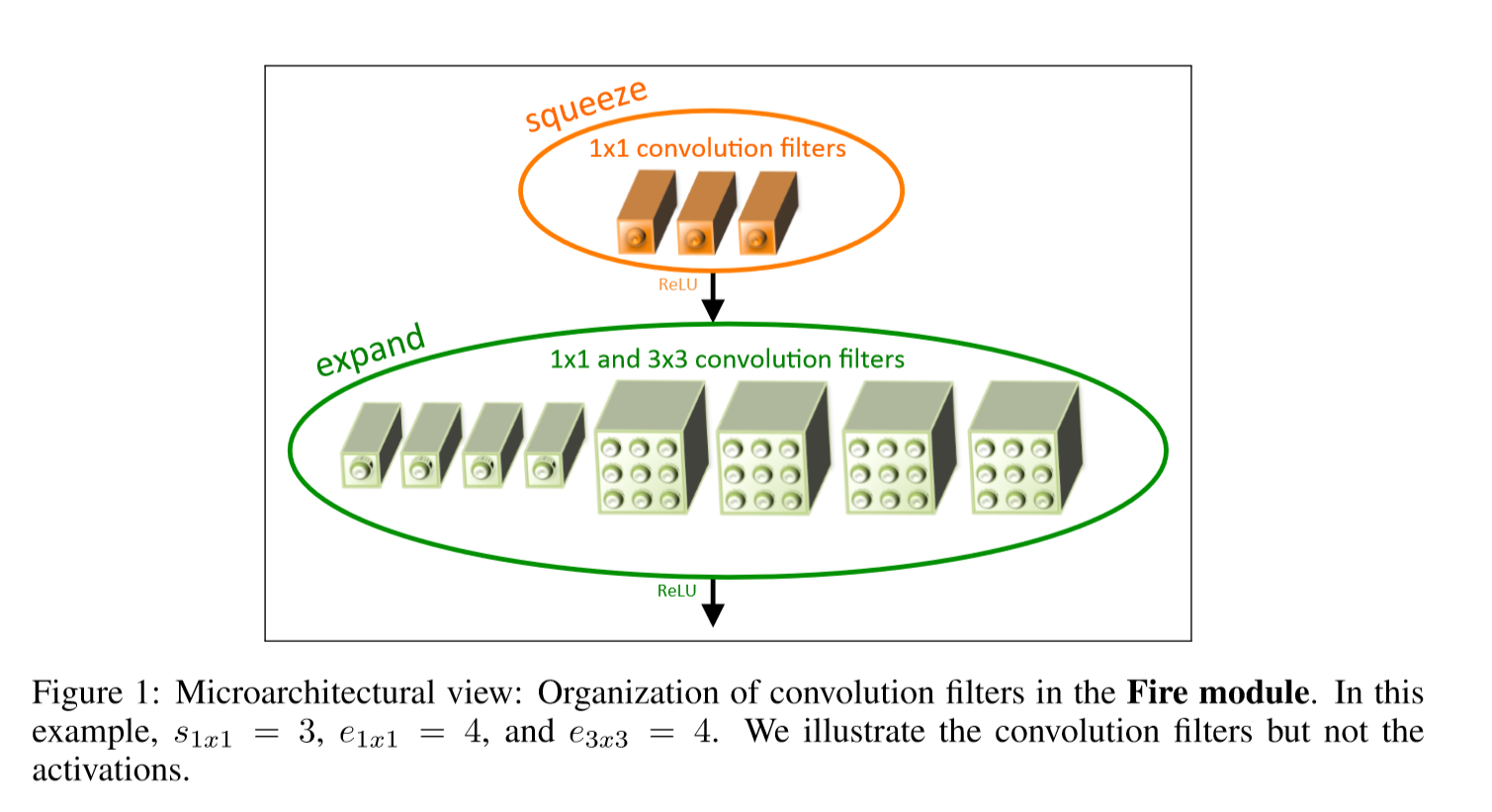
3.2 The Fire Module
A Fire module is comprised of: a squeeze convolution layer (which has only1x1filters), feeding into an expand layer that has a mix of 1x1 and 3x3 convolution filters; we illustrate this in Figure 1.
We expose three tunable dimensions (hyperparameters) in a Fire module: s1x1, e1x1, and e3x3. In a Fire module, s1x1 is the number of filters in the squeeze layer (all 1x1), e1x1 is the number of 1x1 filters in the expand layer, and e3x3 is the number of 3x3 filters in the expand layer. When we use Fire modules we set s1x1 to be less than (e1x1 + e3x3), so the squeeze layer helps to limit the number of input channels to the 3x3 filters.
3.3 The SqueezeNet Architecture
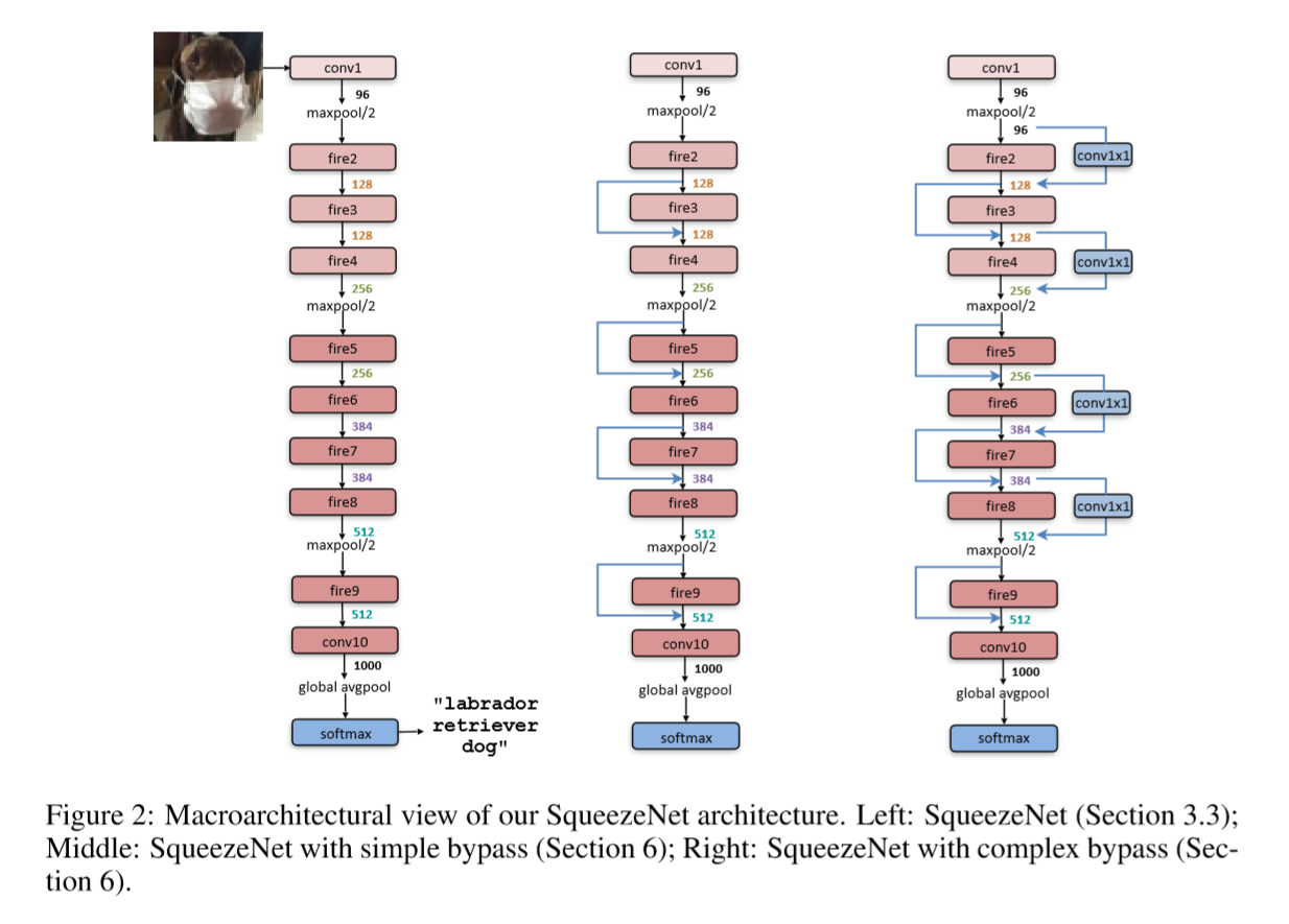
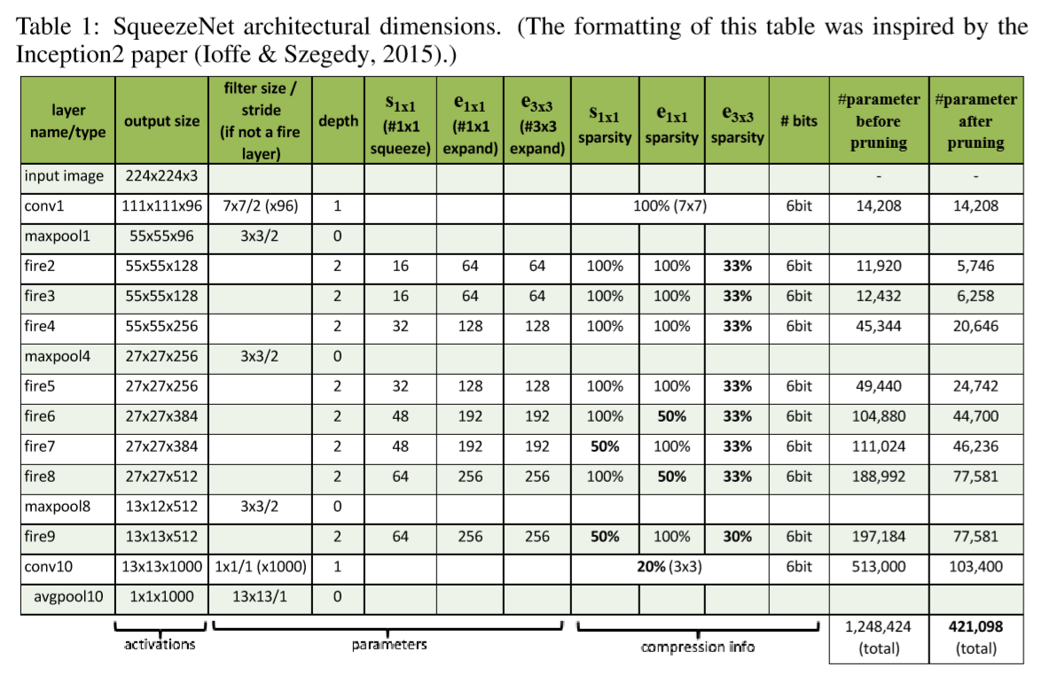
We illustrate in Figure 2 that SqueezeNet begins with a standalone convolution layer (conv1), followed by 8 Fire modules (fire2-9), ending with a final conv layer (conv10). We gradually increase the number of filters per fire module from the beginning to the end of the network. SqueezeNet performs max-pooling with a stride of 2 after layers conv1, fire4, fire8, and conv10; these relatively late placements of pooling are per Strategy 3 from Section 3.1. We present the full SqueezeNet architecture in Table 1.
3.3.1 Other SqueezeNet Details
• So that the output activations from 1x1 and 3x3 filters have the same height and width, we add a 1-pixel border of zero-padding in the input data to 3x3 filters of expand modules.
• ReLU (Nair & Hinton, 2010) is applied to activations from squeeze and expand layers.
• Dropout (Srivastava et al., 2014) with a ratio of 50% is applied after the fire9 module.
• Note the lack of fully-connected layers in SqueezeNet; this design choice was inspired by the NiN (Lin et al., 2013) architecture.
• When training SqueezeNet, we begin with a learning rate of 0.04, and we linearly decrease the learning rate throughout training, as described in (Mishkin et al., 2016). For details on the training protocol (e.g. batch size, learning rate, parameter initialization), please refer to our Caffe-compatible configuration files located here: https://github.com/DeepScale/SqueezeNet.
• The Caffe framework does not natively support a convolution layer that contains multiple filter resolutions (e.g. 1x1 and 3x3) (Jia et al., 2014). To get around this, we implement our expand layer with two separate convolution layers: a layer with 1x1 filters, and a layer with 3x3 filters. Then, we concatenate the outputs of these layers together in the channel dimension. This is numerically equivalent to implementing one layer that contains both 1x1 and 3x3 filters.
We released the SqueezeNet configuration files in the format defined by the Caffe CNN framework. However, in addition to Caffe, several other CNN frameworks have emerged, including MXNet (Chen et al., 2015a), Chainer (Tokui et al., 2015), Keras (Chollet, 2016), and Torch (Collobert et al., 2011). Each of these has its own native format for representing a CNN architecture. That said, most of these libraries use the same underlying computational back-ends such as cuDNN (Chetlur et al., 2014) and MKL-DNN (Das et al., 2016). The research community has ported the SqueezeNet CNN architecture for compatibility with a number of other CNN software frameworks:
• MXNet (Chen et al., 2015a) port of SqueezeNet: (Haria, 2016)
• Chainer (Tokui et al., 2015) port of SqueezeNet: (Bell, 2016)
• Keras (Chollet, 2016) port of SqueezeNet: (DT42, 2016)
• Torch (Collobert et al., 2011) port of SqueezeNet’s Fire Modules: (Waghmare, 2016)
4 Evaluation of SqueezeNet
We now turn our attention to evaluating SqueezeNet. In each of the CNN model compression papers reviewed in Section 2.1, the goal was to compress an AlexNet (Krizhevsky et al., 2012) model that was trained to classify images using the ImageNet (Deng et al., 2009) (ILSVRC 2012) dataset. Therefore,we use AlexNet and the associated model compression results as a basis for comparison when evaluating SqueezeNet.
In Table 2, we review SqueezeNet in the context of recent model compression results. The SVD based approach is able to compress a pretrained AlexNet model by a factor of 5x,while diminishing top-1 accuracy to 56.0% (Denton et al., 2014). Network Pruning achieves a 9x reduction in model size while maintaining the baseline of 57.2% top-1 and 80.3% top-5 accuracy on ImageNet (Han etal.,2015b). Deep Compression achieves a 35x reduction in model size while still maintaining the baseline accuracy level (Han et al., 2015a). Now, with SqueezeNet, we achieve a 50X reduction in model size compared to AlexNet, while meeting or exceeding the top-1 and top-5 accuracy of AlexNet. We summarize all of the aforementioned results in Table 2.
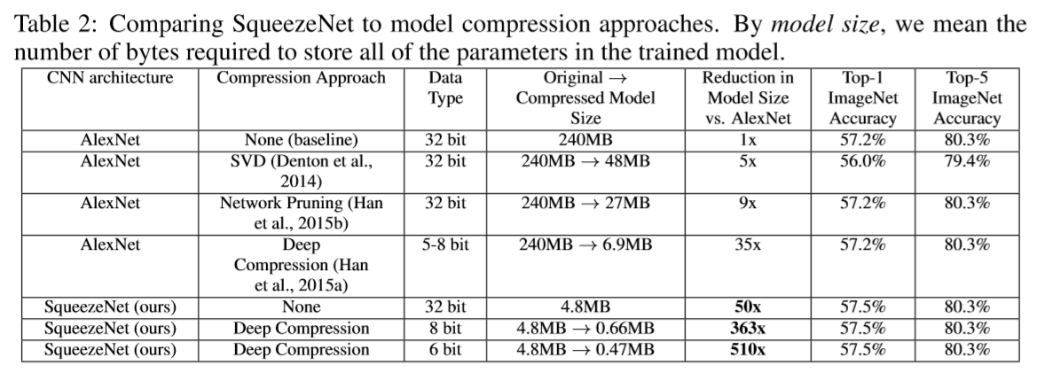
Even when using uncompressed 32-bit values to represent the model, SqueezeNet has a 1.4× smaller model size than the best efforts from the model compression community while maintaining or exceeding the baseline accuracy.
Apply Deep Compression to SqueezeNet, using 33% sparsity and 8-bit quantization. Yield a 0.66 MB model (363× smaller than 32-bit AlexNet) with equivalent accuracy to AlexNet.
Apply Deep Compression with 6-bit quantization and 33% sparsity on SqueezeNet. Produce a 0.47MB model (510× smaller than 32-bit AlexNet) with equivalent accuracy.
Conclusion: Our small model is indeed amenable to compression.
Deep Compression (Han et al., 2015a) not only works well on CNN architectures with many parameters (e.g. AlexNet and VGG), but it is also able to compress the already compact, fully convolutional SqueezeNet architecture
In summary: by combining CNN architectural innovation (SqueezeNet) with state-of-the-art compression techniques (Deep Compression), we achieved a 510×reduction in model size with no decrease in accuracy compared to the baseline.
Finally, note that Deep Compression (Han et al., 2015b) uses a codebook as part of its scheme for quantizing CNN parameters to 6- or 8-bits of precision. Therefore, on most commodity processors, it is not trivial to achieve a speedup of 32 8 = 4x with 8-bit quantization or 32 6 = 5.3x with 6-bit quantization using the scheme developed in Deep Compression. However, Han et al. developed custom hardware – Efficient Inference Engine (EIE) – that can compute codebook-quantized CNNs more efficiently (Han et al., 2016a).
In addition, in the months since we released SqueezeNet, P. Gysel developed a strategy called Ristretto for linearly quantizing SqueezeNet to 8 bits (Gysel, 2016). Specifically, Ristretto does computation in 8 bits, and it stores parameters and activations in 8-bit data types. Using the Ristretto strategy for 8-bit computation in SqueezeNet inference, Gysel observed less than 1 percentage-point of drop in accuracy when using 8-bit instead of 32-bit data types.
5 CNN Microarchitecture Design Space Exploration
Goal: providing intuition about the shape of the microarchitectural design space with respect to the design strategies, understand the impact of CNN architectural choices on model size and accuracy.
5.1 CNN Microarchitecture Metaparameters
In SqueezeNet, each Fire module has three dimensional hyperparameters that we defined in Section 3.2: s1x1, e1x1, and e3x3. SqueezeNet has 8 Fire modules with a total of 24 dimensional hyperparameters.
To do broad sweeps of the design space of SqueezeNet-like architectures, we define the following set of higher level metaparameters which control the dimensions of all Fire modules in a CNN.
basee : the number of expand filters in the first Fire module in a CNN.
After every freq Fire modules, we increase the number of expand filters by incre. That is to say, for Fire Module i, the number of expand filters is
[{e_i} = bas{e_e} + (inc{r_e}*left[ {frac{i}{{freq}}} ight])]
In the expand layer of a Fire module, some filters are 1x1 and some are 3x3; we define ei = ei,1x1 +ei,3x3 with pct3x3 (in the range [0,1],shared over all Fire modules)as the percentage of expand filters that are 3x3.In other words,
[{e_{i,3x3}} = {e_i}*pc{t_{3{ m{x}}3}}] [{e_{i,{ m{1}}x{ m{1}}}} = {e_i}*(1 - pc{t_{3{ m{x}}3}})]
Finally, We defined the squeeze ratio (SR) as the ratio between the number of filters in squeeze layers and the number of filters in expand layers. (again, in the range [0,1], shared by all Fire modules)
[{s_{i,{ m{1}}x{ m{1}}}} = SR*{e_i}]
SqueezeNet (Table 1) is an example architecture that we generated with the aforementioned set of metaparameters. Specifically, SqueezeNet has the following metaparameters: basee = 128, incre = 128, pct3x3 = 0.5, freq = 2, and SR = 0.125.
5.2 Squeeze Ratio
InS ection3.1,we proposed decreasing the number of parameters by using squeeze layers to decrease the number of input channels seen by 3x3 filters. SR
We now design an experiment to investigate the effect of the squeeze ratio on model size and accuracy.
Use SqueezeNet (Figure 2) as a starting point. The metaparameters: basee = 128, incre = 128, pct3x3 = 0.5, and freq = 2.
We train multiple models, where each model has a different squeeze ratio (SR) in the range [0.125, 1.0].
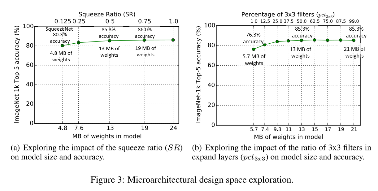
From this figure, we learn that increasing SR beyond 0.125 can further increase ImageNet top-5 accuracy from 80.3% (i.e. AlexNet-level) with a 4.8MB model to 86.0% with a 19MB model. Accuracy plateaus at 86.0% with SR=0.75 (a 19MB model), and setting SR=1.0 further increases model size without improving accuracy.
5.3 Trading off 1x1 and 3x3 Filters
How important is spational resolution in CNN filters?(The spational resolution means the width and the height of the filters)
The VGG (Simonyan & Zisserman, 2014) architectures have 3x3 spatial resolution in most layers’ filters; GoogLeNet (Szegedy et al., 2014) and Network-in-Network (NiN) (Lin et al., 2013) have 1x1filters in some layers. In GoogLeNet and NiN,the authors simply propose a specific quantity of 1x1 and 3x3 filters without further analysis. Here, we attempt to shed light on how the proportion of 1x1 and 3x3 filters affects model size and accuracy.
We use the following metaparameters in this experiment: basee = incre = 128, freq = 2, SR = 0.500, and we vary pct3x3 from 1% to 99%. As in the previous experiment, these models have 8 Fire modules, following the same organization of layers as in Figure 2. We see in Figure3(b) that the top-5 accuracy plateaus at 85.6% using 50% 3x3 filters, and further increasing the percentage of 3x3 filters leads to a larger model size but provides no improvement in accuracy on ImageNet.
6 CNN Macroarchitecture Design Space Exploration
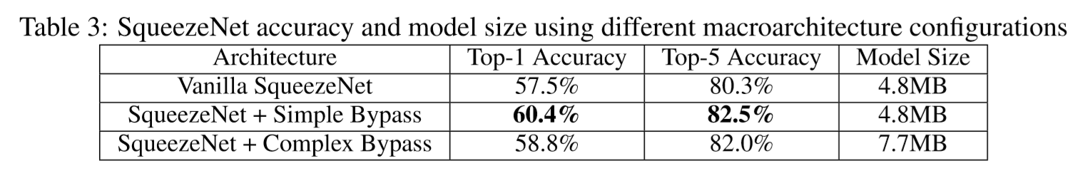
Now, we explore design decisions at the macroarchitecture level concerning the high-level connections among Fire modules. Inspired by ResNet(He et al.,2015b),we explored three different architectures:
• Vanilla SqueezeNet (as per the prior sections).
• SqueezeNet with simple bypass connections between some Fire modules. (Inspired by(Srivastava et al., 2015; He et al., 2015b).)
• SqueezeNet with complex bypass connections between them remaining Fire modules.
We illustrate these three variants of SqueezeNet in Figure 2.
Our simple bypass architecture adds bypass connections around Fire modules 3,5,7,and 9,requiring these modules to learn a residual function between input and output. As in ResNet, to implement a bypass connection around Fire3, we set the input to Fire4 equal to (output of Fire2 + output of Fire3), where the + operator is elementwise addition. This changes the regularization applied to the parameters of these Fire modules, and, as per ResNet, can improve the final accuracy and/or ability to train the full model.
One limitation is that, in the straightforward case, the number of input channels and number of output channels has to be the same( WHY ); as a result, only half of the Fire modules can have simple bypass connections,as shown in the middle diagram of Fig2. When the “same number of channels” requirement can’t be met,we use a complex bypass connection,as illustrated on the right of Figure2. While a simple bypass is “just a wire,” we define a complex bypass as a bypass that includes a 1x1 convolution layer with the number of filters set equal to the number of output channels that are needed. Note that complex bypass connections add extra parameters to the model, while simple bypass connections do not.
In addition to changing the regularization, it is intuitive to us that adding bypass connections would help to alleviate the representational bottleneck introduced by squeeze layers.In SqueezeNet, the squeeze ratio(SR) is 0.125, meaning that every squeeze layer has 8x fewer output channels than the accompanying expand layer. Due to this severe dimensionality reduction, a limited amount of information can pass through squeeze layers. However, by adding bypass connections to SqueezeNet, we open up avenues for information to flow around the squeeze layers.
We trained SqueezeNet with the three macroarchitectures in Figure 2 and compared the accuracy and model size in Table 3. We fixed the microarchitecture to match SqueezeNet as described in Table 1 throughout the macroarchitecture exploration. Complex and simple bypass connections both yielded an accuracy improvement over the vanilla SqueezeNet architecture. Interestingly, the simple bypass enabled a higher accuracy accuracy improvement than complex bypass. Adding the simple bypass connections yielded an increase of 2.9 percentage-points in top-1 accuracy and 2.2 percentage-points in top-5 accuracy without increasing model size.
7 Conclusions
In this paper,we have proposed steps toward a more disciplined approach to the design-space exploration of convolutional neural networks. Toward this goal we have presented SqueezeNet, a CNN architecture that has 50×fewer parameters than AlexNet and maintains AlexNet-level accuracy on ImageNet. We also compressed SqueezeNet to less than 0.5MB, or 510× smaller than AlexNet without compression. Since we released this paper as a technical report in 2016, Song Han and his collaborators have experimented further with SqueezeNet and model compression. Using a new approach called Dense-Sparse-Dense (DSD) (Han et al., 2016b), Han et al. use model compression during training as a regularizer to further improve accuracy, producing a compressed set of SqueezeNet parameters that is 1.2 percentage-points more accurate on ImageNet-1k, and also producing an uncompressed set of SqueezeNet parameters that is 4.3 percentage-points more accurate, compared to our results in Table 2.
We mentioned near the beginning of this paper that small models are more amenable to on-chip implementations on FPGAs. Since we released the SqueezeNet model, Gschwend has developed a variant of SqueezeNet and implemented it on an FPGA (Gschwend, 2016). As we anticipated, Gschwend was able to able to store the parameters of a SqueezeNet-like model entirely within the FPGA and eliminate the need for off-chip memory accesses to load model parameters.
We think SqueezeNet will be a good candidate CNN architecture for a variety of applications, especially those in which small model size is of importance.
SqueezeNet is one of several new CNNs that we have discovered while broadly exploring the design space of CNN architectures.