What is Machine learning?
1. Definition
Definition 1 (older, informal):The field of study that gives computer the ability to learn without being explicitly programmed. – Arthur Samuel
Definition 2 (modern): A computer program is said to learn from experience E with respect to some class of tasks T and performance measure P, if its performance at tasks in T, as measured by P, improves with experience E.– Tom Mitchell
2. Supervised learning & Unsupervised learning
Any machine learning problem can be assigned to one of the 2 broad classifications: supervised learning and unsupervised learning.
Supervised learning: to find out the relationship between the input and the output, given a data set and already know what the correct output should look like.
Can be cauterized into regression problems and classification problems.
Regression problem: to map the input variables to some continuous function.
Classification problem: to map the input variables to discrete categories.
Unsupervised learning: to derive structure from data where we have little or no idea what the results should look like. E.g. clustering, non-clustering.
Linear Regression with one variable
Model Representation & Cost Function
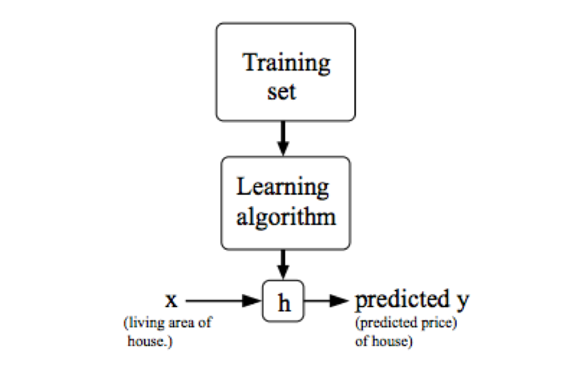
1. model representation
X – The space of input value;
Y– The space of output value;
x’s – input variable / features;
y’s – output variable / target variable;
x(i) – The ith input variable;
y(i) – The ith output value
(x(i), y(i)) – A training example
m – number of training examples;
a list of (x(i), y(i)), i=1, …, m – A training set;
h – hypothesis, a function that maps x’s to y’s.
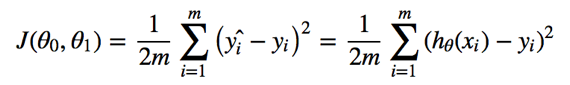
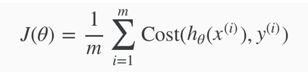
2. cost function
cost function: used to measure the accuracy of the hypothesis function.
 (parameter: θ0, θ1)
a.k.a. squared error function; mean squared error.
Goal –>![]()
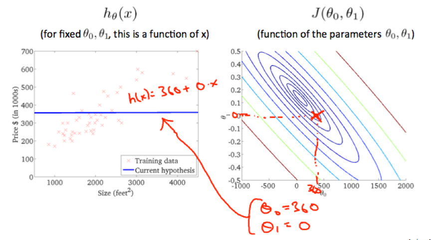
Contour plot: A graph that contains many contour lines. A contour line has a constant value at all points of the same line.
Contour plot can be used to find the parameters that minimize the cost function.
Gradient descent
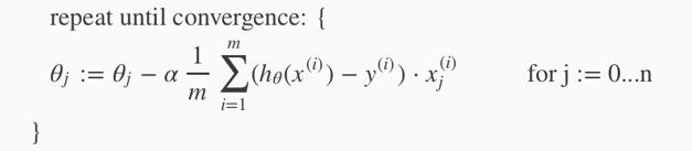
Gradient descent algorithm:
a.k.a. batch gradient descent because it looks at every example in the entire training set
Repeat until convergence {
![]()
} for j=0 and j=1 (i.e. the feature index number)
Depending on where to start on the graph, one could end up at different points.
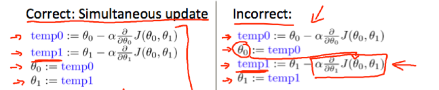
At each iteration, parameters (θ0, θ1, …, θn) should be updated simultaneously.
α – learning rate, a positive number that determines the distance of each step;
α too small -> slow gradient descent.
α too large -> gradient descent fail to converge or even diverge.
The derivative of J(θ0,θ1) determines the direction of gradient descent.
Linear Algebra Review
1. matrix & vector
Dimension of matrix: number of rows * number of columns
Dimension of vector: number of elements in the vector
Aij – i, j entry in the ithrow, jthcolumn of the matrix.
2. Matrix-Vector Multiplication
A× x= y
A– m*n matrix
x– n-dimensional vector
y– m-dimensional vector
multiply A’s ith row with elements of xand add them up to get yi.
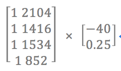
linear prediction = Data Matrix × parameters
e.g. input data {2104, 1416, 1534, 852}, hypothesis h(x)=-40+0.5x, compute the prediction:
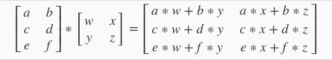
3. Matrix-Matrix Multiplication
A x B = C
A– m*n matrix
B– n*o matrix
C– m*o matrix
Multiply A with the ithcolumn of B to get the ithcolumn of C.
e.g.
Matrices are not commutative: A x B ≠ B x A
Matrices are associative: (A x B) x C =A x (B x C)
Identitiy matrix: n*n matrixIthat has 1’s on the (upper left to lower right) diagonal and 0’s elsewhere.
Ax I= Ix A =A (as long as I’s dimension match A’s row number.)
4. Inverse & Transpose
Inverse: A-1. AA-1= A-1A= I. Can be computed with pinv(A) in octave and inv(A) in Matlab.
Matrices that don’t have an inverse are “singular” or “degenerate”. E.g. matrices with all 0.
A non square matrix does not have an inverse matrix.
Transposition: AT. Aij = ATji. Can be computed with transpose(A) or A’ in matlab.
Linear regression with multiple variables
Multivariate linear regression
1. multiple features
Multivariate linear regression: Linear regression with multiple variables.
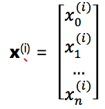
Xj(i) – value of feature j in the ith training example;
X(i) – The features of the ithtraining example;
m – the number of training examples;
n – the number of features;
The hypothesis function hθ(x) = θ0+ θ1x1+ … + θnxn can be represented as:
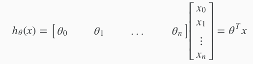 (assume x0(i)=1 for i=1, 2, …, m.)
2. gradient descent for multiple variables
 (simultaneously update θjfor j=0, 1, …, n.)
3. feature scaling & mean normalization
By modifying the ranges of features so that they are roughly on a similar scale so that the gradient descent can converge more quickly.
Feature scaling: dividing the input values by the range of the features, mostly to get every feature into approximately a [-1, 1] range.
e.g.
x1=size (0~2000), x2=number of bedrooms (1~5)
-> x1:=size/2000, x2:=number of bedrooms/5
Mean normalization: replacing xiwith xi-μi to make features have approximately zero mean (do not apply to x0=1), then divide it by the range of value.

xi – the value of a feature;
μ – the average value of the feature (in the training set);
si – the range of the feature. i.e. max-min. can use the standard deviation of the variable instead, but take max-min would be fine, too.
e.g.
xi represents a housing prices with a range of 100 to 2000 and a mean value of 1000
-> xi:=(price-1000)/1900.
4. Debugging gradient descent – how to choose the learning rate
1. (general approach) Plot the cost function J(θ) with the number of gradient descent iterations on the x-axis.
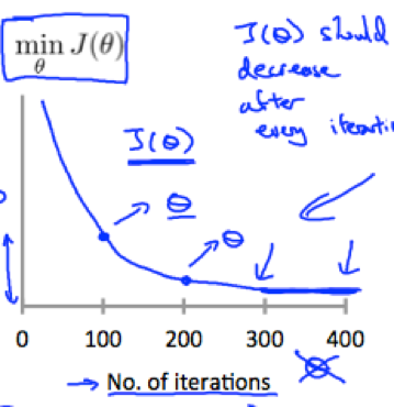
Can help judging whether gradient descent has converged – If gradient descent is working properly (α is sufficiently small), then J(θ) should decrease after every iteration.
αis too small –> gradient descent can be slow to converge.
αis too large -> J(θ) may not decrease on every iteration and thus may not converge.
2. (Alternative approach) Automatic convergence test: Declare convergence if J(θ) decreases by less than a small value E (e.g. 10-3) in one iteration. (but the threshold value is difficult to choose, plotting is preferred.)
5. Polynomial regression
Hypothesis function can be improved by choosing appropriate features in a couples of ways.
1) can combine multiple features into one.
e.g. cobmbine x1and x2into a new feature x3= x1·x2.
2) Polynomial regression (notice that features scaling becomes very important.)
e.g. h(x) = θ0+ θ1x1+ θ2x12+ θ3x13
i.e. set x2=x12, x3=x13, then apply linear regression.
Computing parameters analytically
1. Normal equation
Ways to minimize cost function J:
1) Gradient descent;
2) Normal equation method: A method to solve for θ that minimize J analytically. It takes J’s derivatives with respect to theevery parameter θj in turn and setting them to 0 to solve for θ0, θ1, …, θn.
How to calculate in normal equation method:
We have m training examples (x(1), y(1)), …, (x(m), y(m)) with n features.
yis an m-dimensional vector. Eachx(i)is an (n+1) dimensional feature vector. x0(i)=1
The design matrix: a m*(n+1) matrix 
θ can be calculated by the normal equation formula:
θ=(XTX)−1XTy
Octave: pinv(X’*X)*X’*y
There is no need to do feature scaling with the normal equation.
Comparison
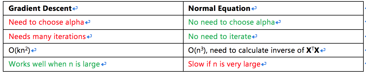
(When n exceeds 10000, it might be a good time to go from normal equation to gradient descent.)
2. normal equation noninvertibility
In Octave, When implementing the normal equation we prefer to use ‘pinv’ (pseudo-inverse) function than ‘inv’. ‘pinv’ will give a right value of θ even if XTX is noninvertible.
If XTX is noninvertible (a.k.a. singular/degenerate)(happens pretty rarely), the common causes might be having:
1) Redundant features; (i.e. two features are linearly dependent.) -> Solution: delete one of the redundant features
2) Too many features (m<=n. m-the number of samples, n-the number of features.) -> Solution: delete some features or use regularization.
Octave/Matlab Tutorial
(Tutorial about operations can reference web pages)
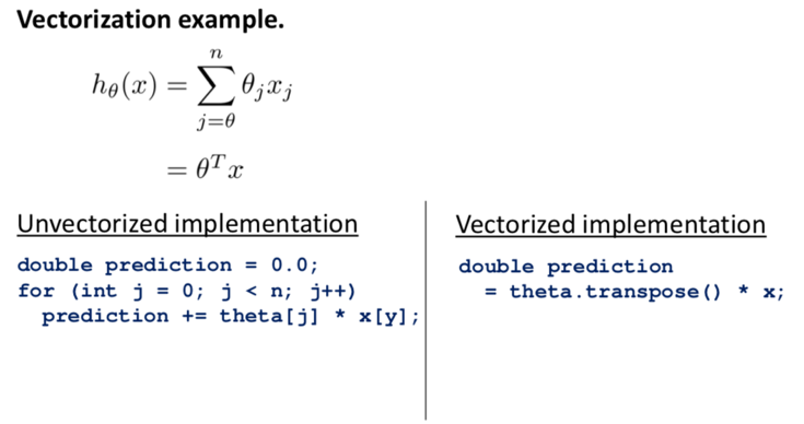
Vectorization
in octave:

can apply to C++ as well:
Vectorized implementation of the update rule of gradient descent(for linear regression):

->


programming hw summarize
in feature scaling, the mean value and standard deviation used in the calculation should be right about the original feature values, not the feature values after some modifications.
e.g. in featureNormalize.m:
mu=mean(X);
sigma=std(X);
X_norm=(X_norm-mu)./sigma; %X_norm is the return value for X
the theta computed by gradient decent and the theta computed by normal equation are different, that's because feature normalization is applied in gradient descent. Thus when predicting with the theta computed by gradient descent, remember to feature normalize the input values first.
e.g.
% Estimate the price of a 1650 sq-ft, 3 br house
x2=[1650, 3];
x2=(x2-mu)./sigma;
x2=[1, x2];
price = x2*theta;
Logistic Regression
Classification & Representation
1. Classification
Binary classification problem: in which the target variable y can take on only 2 values. e.g. 0 (“negative class”) and 1(“positive class”).
Often the negative class is conveying the absence of sth while the positive class conveys the presence of sth, but the it’s still arbitrary and doesn’t matter much.
Multiclass classification problem: in which y may take more than 2 values.
linear regression is not suitable for classification problems.
Logistic Regression: A classification algorithm in which the prediction hθ(x) are always between 0 and 1.
Given x(i), the corresponding y(i) is also called the label for the training example.
2. Hypothesis Representation
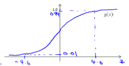
Logistic Function: a.k.a. Sigmoid Function, maps any real number to (0,1).
![]()
the plot of sigmoid function:
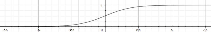
z=0, e0=1 ⇒ g(z)=1/2
z→∞, e−∞→0 ⇒ g(z)=1
z→−∞, e∞→∞ ⇒ g(z)=0
Logistic regression model uses logistic function g to modify hypothesis so that it satisfy0≤hθ(x)≤1.
i.e.

Interpret of hypothesis output
hθ(x) = estimated probability that y=1, given x, parameterized by θ. i.e. hθ(x) = P(y=1 | x;θ)
P(y=0 | x;θ) + P(y=1 | x;θ) = 1.
3. Decision Boundary
In logistic regression:
∵hθ(x)≥0.5 ⇒predict y=1
hθ(x)≤0.5 ⇒predict y=0
and
g(z)≥0.5 when z≥0
∴θTx≥0 ⇒predict y=1
θTx<0 ⇒predict y=0
Decision boundary: the line that separates the area where y=0 and where y=1. Is created by hypothesis function.
The decision boundary is a property of the hypothesis (under the parameters), not a property of the dataset.
We use dataset to fit the parameters, but once we have the parameter vector θthat completely defines the decision boundary, we don’t need to plot a training set in order to plot the decision boundary.
e.g.

In logistic regression, θTx doesn’t have to be linear too, we can add higher order polynomial terms to the features.
Logistic Regression Model
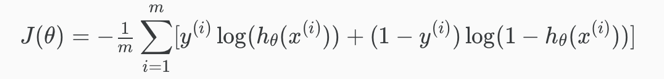
1. Cost Function
Cost function for linear regression:
Cost(hθ(x(i)), y(i)) = 1/2(hθ(x(i))-y(i))2
In logistic regression, we cannot use the same cost function used for linear regression, because the logistic function causes the output to be wavy with many local optima, i.e. not a convex function.
Cost function for logistic regression:
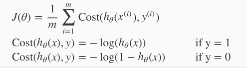
(writing the cost function in this way guarantees that J(θ) is convex for logistic regression.)
Plot:

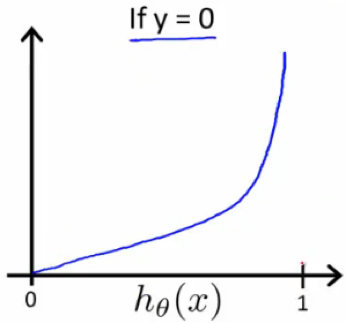
Cost(hθ(x),y)=0 if hθ(x)=y
Cost(hθ(x),y)→∞ if y=0 and hθ(x)→1
Cost(hθ(x),y)→∞ if y=1 and hθ(x)→0
2. Simplified Cost Function and Gradient Descent
Simplified Cost Function
The Cost() function for logistic regression can be compressed into 1 case:
![]()
The entire cost function can be written out as:
Vectorized implementation:
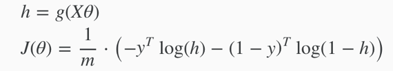
Gradient Descent
The general form of gradient descent:
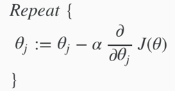
apply the derivative part and get: (still have to simultaneously update all values in theta.)

The update rule is identical to the one used in linear regression, only that the definition of hypothesis has changed.
Vectorized implementation:
![]()
Then get the θ that minimize J(θ). To make prediction on a given new x, output hθ(x).
3. Advanced Optimization
Optimization algorithms can include:
- Gradient Descent;
- Conjugate gradient;
- BFGS;
- L-BFGS.
Conjugate gradient, BFGS and L-BFGS are faster, no need to manually pick α and more sophisticated.
(Suggest not writing these algorithms but use the libraries instead.)
[step 1] write a single function that returns 1) J(θ) and 2) ![]()
function [jVal, gradient] = costFunction(theta)
  jVal = [...code to compute J(theta)...];
  gradient = [...code to compute derivative of J(theta)...];
end
[step 2] call octaves’s advanced optimization functions fminunc() and optimset().
%optimset creates an object containing the options we want to send to fminunc().
%options is a data structure that stores the options you want
%in eg: set the gradient objective parameter to on (confirm that going to provide a gradient)
% and set the maximum number of iterations to 100
options = optimset('GradObj', 'on', 'MaxIter', 100);
% an initial guess for theta
initialTheta = zeros(2,1);
%gice fminunc() our cost function, initial vector of theta values and the options object created.
%@represents a pointer to the function
   [optTheta, functionVal, exitFlag] = fminunc(@costFunction, initialTheta, options);

(notice that Octave use indexes start from 1)
notice that for the Octave implementation, the dimension of theta must >=2.
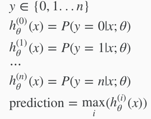
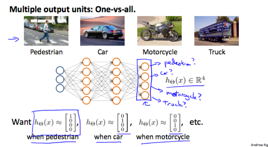
Multiclass Classification: One-vs-all
For classification of data that have more than 2 categories, define y={0, 1, …, n} (start from 0 or 1 doesn’t matter). Divide the problem into n+1 (the number of categories) binary classification problems.
1) Train a logistic regression classifier hθ(x) for each class I to predict the probability that y=i;
(lump all other classes into a single second class)
e.g.
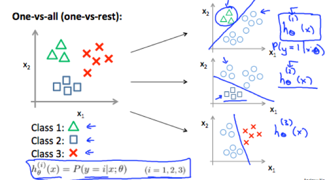
2) To make a prediction on a new x, pick the class that maximize hθ(x).
Regularization
“overfitting”, “underfitting”, and “regularization” can applied to both linear and logistic regression.
Solving the problem of overfitting
1. the problem of overfitting
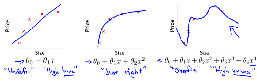
Underfitting: in which hypothesis function maps poorly to the trend of data, is usually caused by a function that is too simple or uses too few features. i.e. the algorithm has high bias.
Overfitting: in which the hypothesis function may fit the training set very well but fails to generalize to predict new data, is usually caused by a complicated function with too many features. i.e. the algorithm has high variance.

Main options to address overfitting:
1) Reduce the number of features:
- Manually select which features to keep.
- Use a model selection algorithm (later in course).
2) Regularization – keep all the features, but reduce the magnitude/values of parameters θj.
Regularization works well when we have a lot of features, each of which contributes a bit to predicting y.
2. cost function
If we have overfitting from our hypothesis function, we can reduce the weight of some terms by increasing their cost.
e.g.
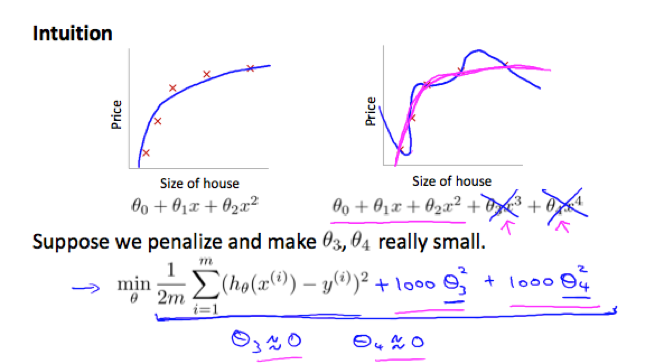
The idea of regularization:
Small values for parameters θ0, θ1, θ0, ..., θngive simpler hypothesis thus less prone to overfitting.
We can add a regularization term (regularize all parameters in a single summation term) to the cost function to shrink all parameters.
By convention the regularization term starts from 1 (not penalizing θ0.)
The cost function for Regularized linear regression:
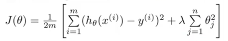
λ – regularization parameter, determines how much the cost of our theta parameters are inflated, controls a trade off between the goal of fitting the data well and the goal of keeping the parameters small (to avoid overfitting).
If lambda is chosen to be too large, it may smooth out the function too much and cause underfitting.
3. regularized linear regression
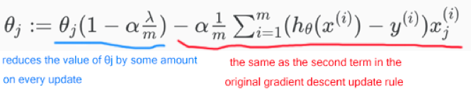
Gradient Decent
In the update rule, Separate out θ0from other parameters because we don’t want to penalize θ0.

can also be represented as:
Normal Equation
Same as the original equation except that adding term λ·L in the (inverse) parentheses.
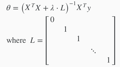
Regularization also solves the problem of non-invertibleXTX
m<n ⇒ XTX is non-invertible/singular (XTX may be non-invertible if m=n)
(can be proved that) λ>0 ⇒ XTX+λ·L is invertible
4. Regularized Logistic Regression
Gradient Descent
the original cost function for logistic regression:
![]()
the cost function for regularized logistic regression:
![]()
![]() means to explicitly exclude the bias term θ0.
means to explicitly exclude the bias term θ0.
Thus when computing θ0 should also be separated from other parameters:
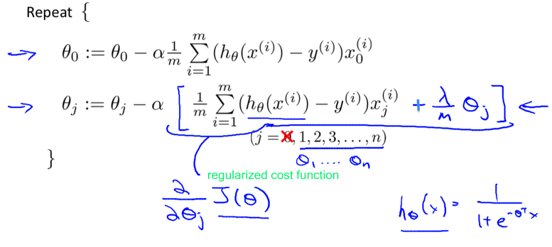
similarly, though the update rule looks the same, it’s not the same algorithm as regularized linear regression because the hypothesis function is different.
Advanced Optimization
[step 1] implement a function[jVal, gradient]=ccostFunction(theta) same as before, just be sure to consider the added term when computing jVal and gradient(2~n+1). (again, notice that Octave uses indexes start from 1)
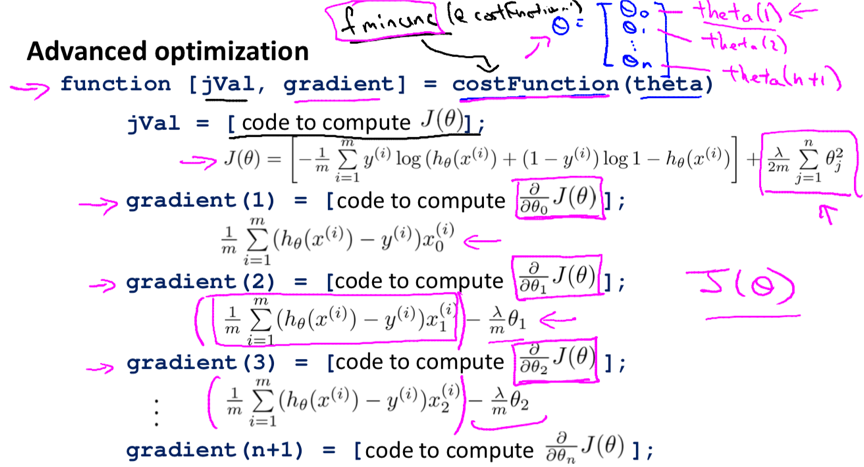
[step 2] pass the function into an advanced optimization function(e.g. fminunc) same as before.
programming hw summarize
when implementing the costFunction() for logistic regression, remember to use sigmoid() when computing the hypothesis, or that the hypothesis could be out of (0,1).
Neural Networks: Representation
Neural Networks
1. Model Representation I
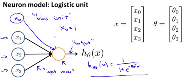
neurons: computational units that take inputs (dendrites: features x1, …, xn. x0is called bias unit, is always equal to 1, sometimes is not drawn.) and channel to outputs (axons: the result of hypothesis function hθ(x)).
In neural networks, we use the same logistic function ![]() (a.k.a. sigmoid (logistic) activation function) as in classification.
(a.k.a. sigmoid (logistic) activation function) as in classification.
θ parameters are sometimes called weights.
e.g. a single neuron with a Sigmoid (logistic) activation function
e.g. neural network

Input layers: input nodes;
Output layer: the node that outputs the hypothesis function;
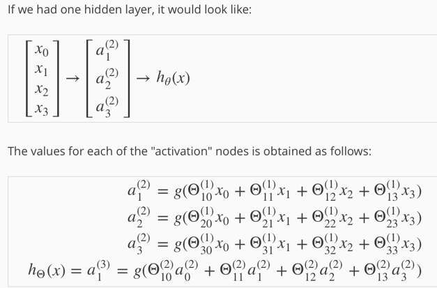
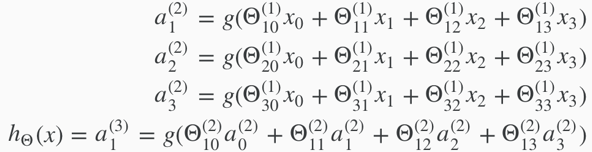
Hidden layers: intermediate layers of nodes between input and output layers. Hidden layer nodes are called activation units, labelled with a0, a1, ..., an.

If network has sj units in layer j and sj+1 units in layer j+1, then Θ(j) will be of dimension sj+1×(sj+1).
The +1 comes from the addition in Θ(j)of the "bias nodes," x0 and Θ0(j).
e.g.
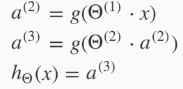
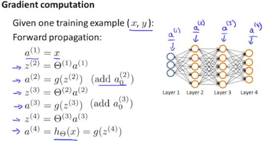
2. Model Representation II
define a new variable zk(j)that encompasses the parameters inside g function.
e.g.
->
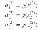
![]()
vectorized implementation
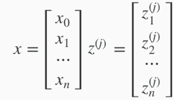 (x0=1)
notice: I think the dimension of z here in the picture should not be n but sj instead, i.e. could be any number >0.
setting x=a(1)
/*then ->*/
z(j)= Θ(j-1)a(j-1)
a(j)= g(z(j)) /*(g is applied element-wise to z(j))*/
/*then add a bias unit a0(j)=1.*/
Θ(j-1): sj*(n+1), sjis the number of activation (a(j)) nodes.
a(j-1): vector with height (n+1).
z(j): vector with height sj. (same height as a(j))
/*The final result suppose j+1 is the output layer, the j here is not the same as the j mentioned above */ hΘ(x)=a(j+1)=g(z(j+1))
The last theta matrix Θj has only 1 row and gets multiplied by column a(j) so the result is a single number. In the last step, what we are doing exactly the same thing as we did in logistic regression, just that the features fed into logistic regression are values computed by hidden layers (e.g. a1, a2, a3…).
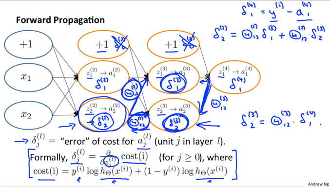
This process of computinghΘ(x)is called forward propagation.
Architectures: how the different neurons are connected to each other.
Applications
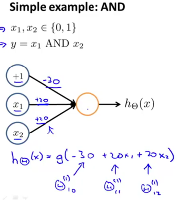
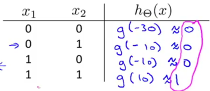
1. Examples and Intuitions I
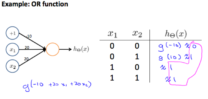
Neural network can compute a complex non-linear function of the input. E.g. Neural networks can be used to simulate logical gates.
g(z) is like:
x1 AND x2
x1 OR x2
2. Examples and Intuitions II
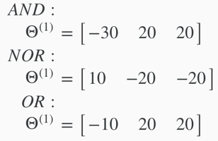
NOT x1 idea: put a large negative weight in front of the variable you want to negate

we can combine AND, NOR and OR to get the XNOR logical operator:
The Θ(1) matrices for AND, NOR, and OR:
XNOR
![]()
![]()
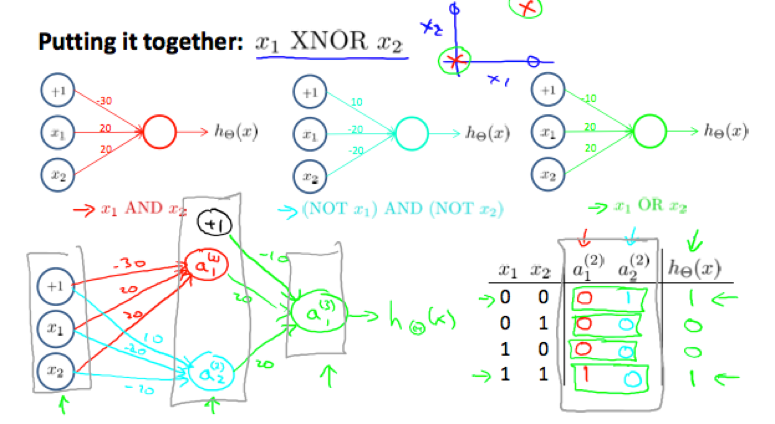
In neural network with multiple layers, a layer can build on the simpler previous layer to complete more complex functions.
3. Multiclass Classification
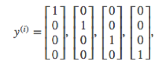
to do multiclass classification in neural network, we let the hypothesis function return a vector of values.
e.g.
original: y∈{1,2,3,4}
->
neural network:

Neural Networks: Learning
Cost Function and Backpropagation
1. Cost Function – how to compute cost function
L – total number of layers in the network;
sl – number of units (not counting bias unit) in layer l;
K – number of units in the output layer.
Binary classification has only 1 output unit (sL=1) –> y=0 or 1, hΘ(x) is a real number.
Multiclass classification (K classes, K>=3) has K output units (sL=K) -> hΘ(x) is a k-dimensional vector.
hΘ(x)k – the hypothesis that results in the kth output;
cost function for regularized logistic regression:
![]()
cost function for neural networks: add nested summations to account for multiple output nodes.

(K=1 when it’s a binary classification problem.)
the double sum simply adds up the logistic regression costs calculated for each cell in the output layer;
the triple sum simply adds up the squares of all the individual Θ(l)jis (except those corresponding to the bias units i.e. when i=0) in the entire network. (there are multiple theta matrices).(the i in the triple sum does not refer to training example i.)
For a theta matrix:
number of columns = number of nodes in current layer, including the bias unit;
number of rows = number of nodes in the next layer, excluding the bias unit.
2. Backpropagation Algorithm – how to compute partial derivative term
L – the total number of layers in the network;
δj(L) – the error of node j in layer l, is written in vectorization below. There is no δ(1).
a(l).*(1-a(l)) – is actually the derivative of the activation function evaluated at the input values given by z(l): ![]()
Given training set {(x(1), y(1)), …, (x(m), y(m))}
Set ![]() for all (l,i,j).
for all (l,i,j).
For training example t=1 to m:
1) Set
![]()
2) Perform forward propagation to compute a(l) for l=2, 3, …, L.
3) compute δ(L) using
![]() (with vectorization)
(with vectorization)
4) Compute δ(L−1), δ(L−2), …,δ(2) using
![]()
and update delta matrix Δ
![]() or with vectorization,
or with vectorization, ![]()
End of traversal
(go outside the loop) update capital-delta matrix D
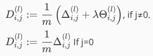 (D works as an accumulator.)
Finally, compute the partial derivative using
![]()
3. Backpropagation Intuition
If we consider non-multiclass classification and disregard regularization,
Backpropagation in Practice
1. Implementation Note: Unrolling Parameters
function [jVal, gradient] = costFunction(theta);
…
optTheta = fminunc(@costFunction, initialTheta, options);
Optimizing functions (such as Fminunc()) assume that parameter theta, initialTheta, and returned value gradient are vectors, while in neural networks they are matrices, so we need to unroll matrices Θ(l), D(l) into long vectors.
e.g. for neural network L=4.
thetaVector = [ Theta1(:); Theta2(:); Theta3(:); ]
deltaVector = [ D1(:); D2(:); d3(:) ]
To get back the original matrices from the unrolled vector:
e.g. if the dimensions of Theta1 is 10*11, Theta2 is 10*11 and Theta3 is 1*11.
Theta1 = reshape(thetaVector(1:110),10,11)
Theta2 = reshape(thetaVector(111:220),10,11)
Theta3 = reshape(thetaVector(221:231),1,11)
To summarize:
Have initial parameters Θ(1),Θ(2),Θ(3), … .
-> Unroll these theta parameters to get a vector initialTheta to pass to fminunc(@costFunction, initialTheta, options).
-> Implement function [jVal, gradientVec] = costFunction(thetaVec), in which thetaVec has been unrolled into a vector:
1) reshape thetaVec to get original parameter matrices Θ(1),Θ(2),Θ(3), … .
2) Use these parameter matrices to run forward/back propagation to compute derivatives D(1), D(2), D(3), … and cost J(Θ).
3) Unroll D(1), D(2), D(3), … to get vector gradientVec that should be returned.
2. Gradient Checking
Gradient checking can assure that our backpropagation works as intended.
The derivative of cost function can be approximated with: (two-sided difference, is more accurate than one-sided difference estimate.)
![]() (when Θis a real number)
(when Θis a real number)
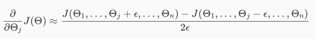 (when Θ∈Rnis the unrolled version of multiple matrices Θ(1), Θ(2),Θ(3), …)
ϵ - a small value such as 10-4.
Octave implementation:
epsilon = 1e-4;
for i = 1:n, /*n is the dimension of the unrolled version of Θ*/
  thetaPlus = theta;
  thetaPlus(i) += epsilon;
  thetaMinus = theta;
  thetaMinus(i) -= epsilon;
  gradApprox(i) = (J(thetaPlus) - J(thetaMinus))/(2*epsilon)
end;
Implementation Note:
1) Implement backpropagation to compute deltaVector(unrolled D(1), D(2), D(3), …);
2) Implement numerical gradient checking to compute gradApprox;
3) Check if gradApprox ≈ deltaVector;
4) Turn off gradient checking before continuing training the classifier with backpropagation. (because the code to compute gradApprox is very slow, backpropagation is a much faster way to compute derivatives than gradient checking.)
3. Random Initialization – symmetric breaking
Before backpropagation,initializing all theta weights to 0 does not work with neural networks because all nodes will update to the same value repeatedly.
We can randomly initialize Θ matrices by: (the epsilon used here is unrelated to the epsilon from gradient checking)

Octave implementation:
/* If the dimensions of Theta1 is 10x11, Theta2 is 10x11 and Theta3 is 1x11.
rand(x,y) is used to initialize a matrix of random real numbers between 0 and 1. */
Theta1 = rand(10,11) * (2 * INIT_EPSILON) - INIT_EPSILON;
Theta2 = rand(10,11) * (2 * INIT_EPSILON) - INIT_EPSILON;
Theta3 = rand(1,11) * (2 * INIT_EPSILON) - INIT_EPSILON;
4. Putting it together
How to pick a network architecture:
Number of input units: dimension of features x(i);
Number of output units: number of classes;
Number of hidden layers: 1 as defaults, or if >1, recommend to have the same number of units in every hidden layer;
Number of hidden units per layer: usually the more the better, but must balance with the cost of computation.
The overall process of training a neural network learning algorithm
1) Randomly initialize the weights;
2) Implement forward propagation to get hΘ(x(i)) for any x(i);
3) Implement the code to compute cost function;
4) Implement backpropagation to compute partial derivatives;
Usually use a loop over the training examples:
for i = 1:m,
   Perform forward propagation and backpropagation using example (x(i),y(i))
   (Get activations a(l) and delta terms d(l) for l = 2,...,L).
Then compute the partial derivatives term outside the loop.
5) Use gradient checking to confirm that your backpropagation works. Then disable gradient checking.
6) Use gradient descent or advanced optimization method to minimize J(Θ) as a function of theta.
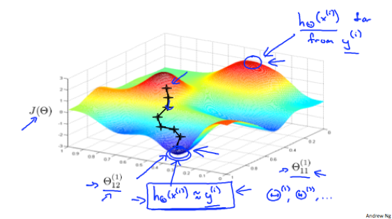
Notice: In neural network J(Θ) is not convex thus we might end up in a local optimum.
An intuition of what gradient descent for a neural network is doing:
Advice for Applying Machine Learning
Evaluating a Learning Algorithm
1. Deciding What to Try Next
Possible ways to try next when the current prediction is making large errors:
- Get more training examples;
- smaller set of features;
- getting additional features;
- adding polynomial features;
- decreasing λ;
- increasing λ.
Machine learning diagnostic: A test that can run to gain insight what is/isn’t working with a learning algorithm, and gain guidance as to how best to improve its performance.
2. Evaluating a Hypothesis
To evaluate a learned hypothesis,
split up the given dataset of training examples into 2 sets: a training set (70%) and a test set (30%) (if the data is in some order, split them into 70%, 30% after randomly sorting.), then:
1) Learn Θ from the training set;
2) compute the test set error Jtest(Θ).
For linear regression:
Test set error: ![]()
For classification:
Test set error: ![]()
An alternative test sets metric: Misclassification error, a.k.a. 0/1 misclassification error
![]()
Then define the test error using the misclassification error: (it gives the proportion of the misclassified test data)
![]()
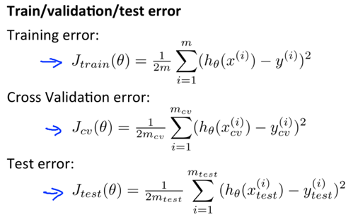
3. Model Selection & Train/Validation/Test Sets
Model Selection: To choose a model (i.e a degree of polynomial or regularization parameter lambda) for the hypothesis.
Problem -> if fitting the degree of polynomial d using the test set, then JtestΘ(d)is likely to be an overly optimistic estimate of generalization error.
Solution -> to get d that has not been trained using the test set:
Split the dataset into 3 sets: training set (60%), cross validation set (20%), and test set (20%), then:
1) Optimize Θ using the training set for each polynomial degree;
2) Find d with the least error using the cross validation set;
3) Estimate the generalization error Jtest(Θ(d)) using the test set.
Bias vs. Variance
1. Diagnosing Bias vs. Variance
To distinguish whether bias or variance is the problem contributing to the bad predictions:

High bias (underfitting): both Jtrain(Θ) and JCV(Θ) are high, Jtrain(Θ)≈Jtrain(Θ).
High variance (overfitting): Jtrain(Θ) is low, JCV(Θ) is much higher than Jtrain(Θ).
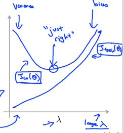
2. Regularization and Bias/Variance
To choose a suitable regularization parameter λ,
(Jtrain, JCV and Jtest are all computed without the extra regularization term.)
1) Create a list of λ (e.g. λ∈{0,0.01,0.02,0.04,0.08,0.16,0.32,0.64,1.28,2.56,5.12,10.24});
2) Create a set of models with different degrees or any other variants;
3) Learn Θ for each model with different λ;
4) Compute the cross validation error JCV(Θ) using the learned Θ, without regularization term;
5) Select the best combo (Θ and λ) that produces the lowest error on cross validation set;
6) apply the selected Θ and λ on Jtest(Θ) to see if it has a good generalization of the problem.
3. Learning Curves - to plot Jtrain(Θ) and JCV(Θ) (without regularization), can help to diagnose whether the algorithm is suffering from high bias or high variance.
High bias:
Low training set size -> low Jtrain(Θ), high JCV(Θ);
Large training set size -> Jtrain(Θ)≈JCV(Θ), both are high.
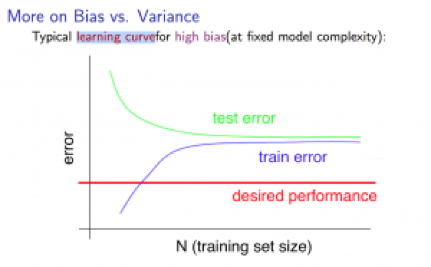
notice: I think the “test error” in the picture (and the picture below) should be “cross validation error”instead, but test error just applies as well, anyway.
If a learning algorithm is suffering from high bias, getting more training data will not help much.
High variance:
Low training set size -> low Jtrain(Θ), high JCV(Θ);
Large training set size -> Jtrain(Θ) increases, JCV(Θ) decreases without levelling off. Jtrain(Θ)< JCV(Θ) but the difference between them remains significant.
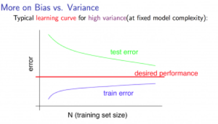
If a learning algorithm is suffering from high variance, getting more training data is likely to help.
4. Deciding What to Do Next Revisited
The decision of which way to choose to improve the prediction can be made based on the variance/bias of the current algorithm.
- Get more training examples – Fixes high variance;
- smaller set of features – Fixes high variance;
- getting additional features – Fixes high bias;
- adding polynomial features – Fixes high bias;
- decreasing λ – Fixes high bias;
- increasing λ – Fixes high variance.
Diagnosing Neural Networks
Neural network with fewer parameters -> prone to underfitting, computationally cheaper;
Neural network with more parameters (more hidden units/layers) -> prone to overfitting, computationally expensive. [We can use regularization (increase λ) to address overfitting].
Usually, a larger neural network with regularization is more effective than a smaller neural network.
Using a single hidden layer -> usually a Reasonable default.
Using a number of hidden layers -> we can train neural network on different number of hidden layers, see then select the one that performs best on the cross-validation sets .
Model Complexity Effects
Lower-order polynomials (low model complexity) -> high bias, low variance, the model fits poorly consistently;
Higher-order polynomials (high model complexity) -> low bias (on training data), high variance, fit the training data well but the test data poorly;
In reality we would want to choose a model somewhere in between.
Machine Learning System Design
Building a Spam Classifier
1. Prioritizing What to Work On
To build a spam classifier we can:
construct a vector (feature x) for each email, each entry represents a word indicative of spam/not spam.
x(i)=1 if word(i) is found in the email, else 0;
In practice, the vector normally contains 10,000 to 50,000 entries gathered by finding the most frequently used words in the training set.
label y=1 if the email is spam, else 0.
Some options to spend time on to improve the accuracy of accuracy of the built classifier: (It’s difficult to tell which will be most helpful)
1) Collect lots of data (e.g. “honeypot” project: create fake email addresses used to collect a lot of spam emails. But doesn’t not always work.);
2) Develop sophisticated features based on email routing information (from using email header data in spam emails);
3) Develop sophisticated features for message body (e.g. treat “discount”/”discounts”, “deal”/”dealer”as the same word? Feature about punctuation? );
4) Develop sophisticated algorithms to process the input in different ways (e.g. recognizing misspelling in spam);
2. Error Analysis
The recommended approach to solve machine learning problem:
- Start with a simple algorithm, implement it quickly, and test it early on the cross validation set;
- Plot learning curves to decide if more data, more features, etc. are likely to help;
- Manually examine the errors on examples in the cross validation set, and try to spot a trend where most of the errors were made. -> often inspire you to find the current shortcoming and come up with improvements.
e.g. error analysis for spam classifier:
Manually examine the misclassified emails, categorize them based on 1) email type 2) what cues you think would have helped the algorithm classify them correctly
-> by seeing the ratio of types/features in the misclassified emails, we could add some particular new features to the model.
Recommendation: do the error analysis on the cross validation set rather than the test set.
Numerical evaluation: A single numerical value (real number) that tells how well the algorithm is doing. E.g. cross validation error.
Problem:Error analysis may not be helpful for deciding if this is likely to improve performance.
Solution: try the new idea (drawn from the error analysis) quickly, compare the numerical evaluation of the algorithm’s performance with and without the modification, see if it works.
Handling Skewed Data
1. Error Metrics for Skewed Classes
skewed classes: where the ratio of positive to negative examples is very close to one of the two extremes.
Problem: For skewed classes, a bad algorithm that predicting y=0 or y=1 all the time can behave well on evaluation metric such as classification error or classification accuracy.
Solution: use precision/recall as evaluation metric so that such algorithms cannot get a high performance.
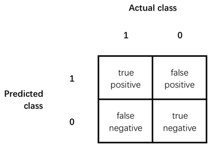
Precision: Of all the examples we predicted y=1, what fraction actually y=1?
![]()
Recall: Of all the examples that actually y=1, what fraction did we correctly predict y=1?
![]()
Accuracy = (true positives + true negatives) / (total examples)
When defining precision and recall, we usually define y=1 in presence of rare class that we want to detect.
2. Trading Off Precision and Recall
Classifiers can vary the threshold to control trade off between precision and recall.
Logistic regression predict y=1 if hθ(x)>=threshold.
Usually -> threshold=0.5;
Want higher precision, lower recall -> higher threshold (predict y=1 only if very confident);
Want lower precision, higher recall -> lower threshold (avoid missing too many y=1).
By varying the threshold, we can plot a precision-recall curve for the algorithm:
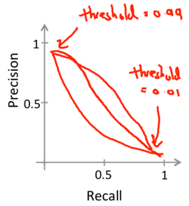
The shape of the curve depends on the details of the classifier.
How to compare algorithms based on precision/recall
The average (P+R)/2 is not a good way to evaluation algorithms.
F1 Score: a.k.a. F score. A good way to combine precision and recall. For the F Score to be large, both P and R have to be large.
![]()
A reasonable way to pick a threshold:
1) try a range of different thresholds;
2) evaluate the classifiers by F score on the cross-validation set;
3) pick the threshold that gives the highest F score.
Using Large Data Sets
Under certain conditions, getting a lot of training data is an effective way get a high-performance learning algorithm.
1. feature x has sufficient information to predict y accurately.
-> Useful test: Given the same input x, can a human expert confidently predict y?
2. The learning algorithm has many parameters. E.g. logistic regression/linear regression with many features, neural network with many hidden units.
Reasons:
Has many parameters -> low bias, Jtrain(θ) will be small.
Use a large training set -> low variance, Jtrain(θ)≈Jtest(θ). (unlikely to overfit)
-> Jtest(θ) will be small.