线性回归和局部加权线性回归

线性回归

算法优缺点：

优点：结果易于理解，计算不复杂
缺点：对非线性数据拟合不好
适用数据类型：数值型和标称型

算法思想：

这里是采用了最小二乘法计算（证明比较冗长略去）。这种方式的优点是计算简单，但是要求数据矩阵X满秩，并且当数据维数较高时计算很慢；这时候我们应该考虑使用梯度下降法或者是随机梯度下降（同Logistic回归中的思想完全一样，而且更简单）等求解。这里对估计的好坏采用了相关系数进行度量。

数据说明：

这里的txt中包含了x0的值，也就是下图中前面的一堆1，但是一般情况下我们是不给出的，也就是根据一个x预测y，这时候我们会考虑到计算的方便也会加上一个x0。

数据是这样的

函数：

loadDataSet(fileName):
读取数据。
standRegres(xArr,yArr)
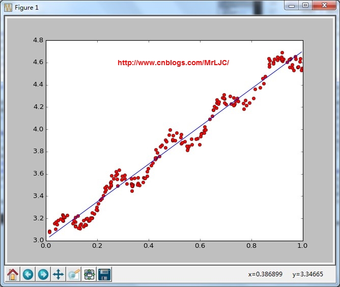
普通的线性回归，这里用的是最小二乘法

plotStandRegres(xArr,yArr,ws)
画出拟合的效果
calcCorrcoef(xArr,yArr,ws)
计算相关度，用的是numpy内置的函数

结果：

局部加权线性回归（Locally Weighted Linear Regression）

算法思想：

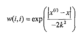
这里的想法是：我们赋予预测点附近每一个点以一定的权值，在这上面基于最小均方差来进行普通的线性回归。这里面用“核”（与支持向量机相似）来对附近的点赋予最高的权重。这里用的是高斯核：

函数：

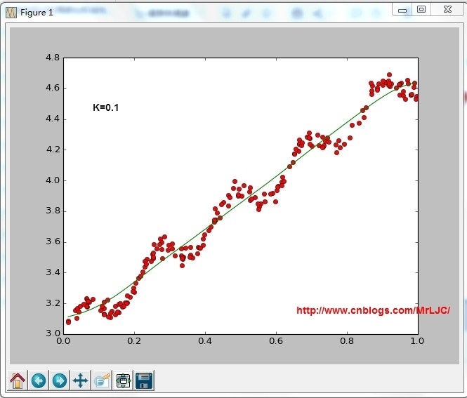
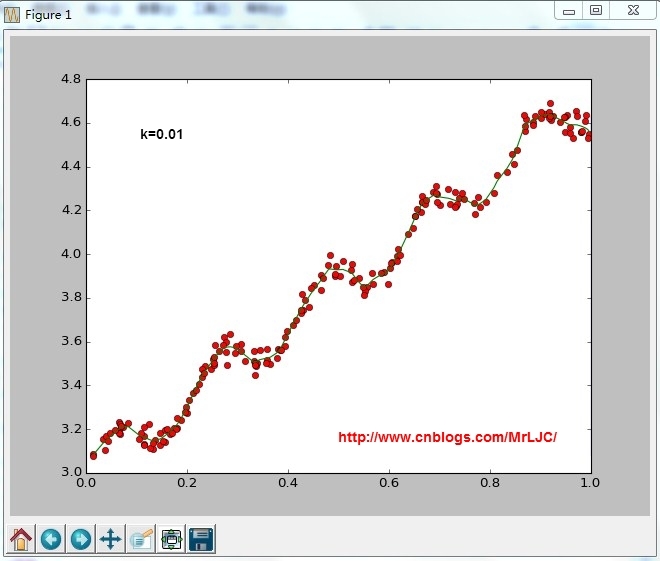
lwlr(testPoint,xArr,yArr,k=1.0)
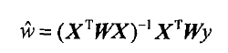
根据计算公式计算出再testPoint处的估计值，这里要给出k作为参数，k为1的时候算法退化成普通的线性回归。k越小越精确（太小可能会过拟合）求解用最小二乘法得到如下公式：

lwlrTest(testArr,xArr,yArr,k=1.0)
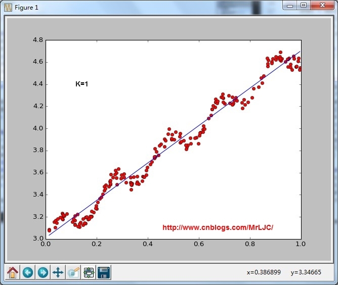
因为lwlr需要指定每一个点，这里把整个通过循环算出来了
lwlrTestPlot(xArr,yArr,k=1.0)
将结果绘制成图像

结果：

 1 from numpy import *
 2 def loadDataSet(fileName):
 3     numFeat = len(open(fileName).readline().split('	')) - 1 
 4     dataMat = []; labelMat = []
 5     fr = open(fileName)
 6     for line in fr.readlines():
 7         lineArr =[]
 8         curLine = line.strip().split('	')
 9         for i in range(numFeat):
10             lineArr.append(float(curLine[i]))
11         dataMat.append(lineArr)
12         labelMat.append(float(curLine[-1]))
13     return dataMat,labelMat
14 def standRegres(xArr,yArr):
15     xMat = mat(xArr)
16     yMat = mat(yArr).T
17     xTx = xMat.T * xMat
18     if linalg.det(xTx) == 0.0:
19         print 'This matrix is singular, cannot do inverse'
20         return
21     ws = xTx.I * (xMat.T * yMat)
22     return ws
23 def plotStandRegres(xArr,yArr,ws):
24     import matplotlib.pyplot as plt 
25     fig = plt.figure()
26     ax = fig.add_subplot(111)
27     ax.plot([i[1] for i in xArr],yArr,'ro')
28     xCopy = xArr
29     print type(xCopy)
30     xCopy.sort()
31     yHat = xCopy*ws
32     ax.plot([i[1] for i in xCopy],yHat)
33     plt.show()
34 def calcCorrcoef(xArr,yArr,ws):
35     xMat = mat(xArr)
36     yMat = mat(yArr)
37     yHat = xMat*ws
38     return corrcoef(yHat.T, yMat)
39 def lwlr(testPoint,xArr,yArr,k=1.0):
40     xMat = mat(xArr); yMat = mat(yArr).T
41     m = shape(xMat)[0]
42     weights = mat(eye((m)))
43     for j in range(m):
44         diffMat = testPoint - xMat[j,:]
45         weights[j,j] = exp(diffMat*diffMat.T/(-2.0*k**2))
46     xTx = xMat.T * (weights * xMat)
47     if linalg.det(xTx) == 0.0:
48         print "This matrix is singular, cannot do inverse"
49         return
50     ws = xTx.I * (xMat.T * (weights * yMat))
51     return testPoint * ws
52 def lwlrTest(testArr,xArr,yArr,k=1.0):
53     m = shape(testArr)[0]
54     yHat = zeros(m)
55     for i in range(m):
56         yHat[i] = lwlr(testArr[i],xArr,yArr,k)
57     return yHat
58 def lwlrTestPlot(xArr,yArr,k=1.0):
59     import matplotlib.pyplot as plt
60     yHat = zeros(shape(yArr))
61     xCopy = mat(xArr)
62     xCopy.sort(0)
63     for i in range(shape(xArr)[0]):
64         yHat[i] = lwlr(xCopy[i],xArr,yArr,k)
65     fig = plt.figure()
66     ax = fig.add_subplot(111)
67     ax.plot([i[1] for i in xArr],yArr,'ro')
68     ax.plot(xCopy,yHat)
69     plt.show()
70     #return yHat,xCopy
71 def rssError(yArr,yHatArr): #yArr and yHatArr both need to be arrays
72     return ((yArr-yHatArr)**2).sum()
73 def main():
74     #regression
75     xArr,yArr = loadDataSet('ex0.txt')
76     ws = standRegres(xArr,yArr)
77     print ws
78     #plotStandRegres(xArr,yArr,ws)
79     print calcCorrcoef(xArr,yArr,ws)
80     #lwlr
81     lwlrTestPlot(xArr,yArr,k=1)
82 if __name__ == '__main__':
83     main()

机器学习笔记索引

来自为知笔记(Wiz)