源地址(相关案例在视频下方): http://cookdata.cn/auditorium/course_room/10018/
《机器学习十讲》——第七讲(最优化)
机器学习的优化目标
最小化损失函数: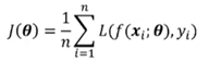
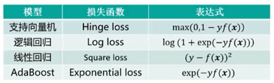
模型——损失函数——表达式:
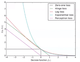
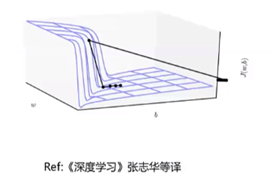
图示:
方法
梯度下降:
batch梯度下降:使用全部训练集样本,计算代价太高(n~10^6)
mini-batch梯度下降:随机采样一个子集(m~100或1000),随后使用如下公式: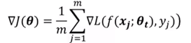
mini-batch是无偏估计。更大的批量会减小梯度计算的方差。
随机梯度下降SGD:
使用mini-batch计算出结果后再根据梯度下降法的公式: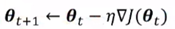 去更新参数,下一步再随机采样子集,重复该操作。此方法称为随机梯度下降(SGD)。
因此有说法:mini-batch是SGD的推广,通常所属SGD即是mini-batch。
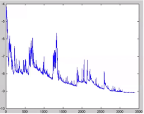
因为是训练一次样本更新一次参数,所以梯度下降时通常呈振荡的形式,但大方向上还是下降趋势:
在SGD中学习率的设定是关键。
理论上保证SGD收敛的充分条件:  。因此需要随着迭代次数的增加降低学习率。
设定学习率的方法:

梯度下降在实际应用中的问题
病态条件:

右图:假设周边都是悬崖,那么在进行梯度下降算法时会出现垂直下降的情况。
局部最小与全局最小:
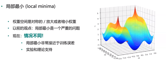
右图所示,直观可以看出最小值在第三个凹处,然而在实际算法中根据设定起点不同,得到的“最小值”可能不是全局最小。
鞍点:
梯度为0,Hessian矩阵同时存在正值和负值;Heissan矩阵的所有特征值为正值的概率很低;对于高维情况,鞍点和局部最小点的数量多。如图所示:

在使用二阶优化算法会有问题。
平台:
梯度为0,Hessian矩阵也为0。如图所示:
需要加入噪音使得从平台区域跳出。
梯度爆炸与悬崖:
在RNN中非常常见,参数不断相乘导致;长期时间依赖性。如图所示:
解决方法:梯度截断,启发式梯度截断干涉以减少步长。
SGD方法改进:
动量法:
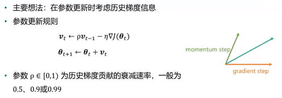
ρ可以随着迭代次数的增大而变大,随着时间推移调整ρ比收缩η更重要。
动量法克服了SGD中的两个问题:
Hessian矩阵的病态问题(图示):
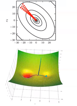
随机梯度的方差带来的不稳定。
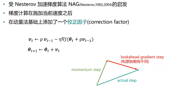
Nesterov动量法:
AdaGrad:
学习率自适应:与梯度历史平方值总和的平方根成反比。
效果:更为平缓的倾斜方向上会取得更大的进步,可能逃离鞍点。
问题:累积梯度平方和增长过快,导致学习率迅速较小,提前终止学习。
公式: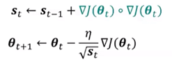
RMSProp:
在AdaGrad基础上,降低了对早期历史梯度的依赖;通过设置衰减系数β2实现(建议β2=0.9)
公式:
Adam:
同时考虑动量和学习率自适应。β1通常设置成0.9,β2设置成0.999
公式: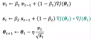
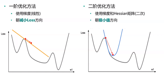
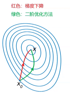
二阶优化方法:
与一阶优化方法的比较
牛顿法:使用二阶泰勒展开: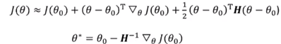
通常Hessian矩阵(H^-1)不是正定的,增加正则化策略:![]()
对于高维情形,代价太高,需要近似:L-BFGS方法。
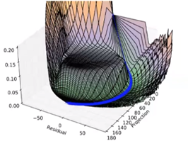
二阶优化方法与梯度下降的图示比较:
优化算法选择
在大数据场景(样本量大,特征维数大)下,一阶方法最实用(随机梯度)。
自适应学习率算法族(以RMSProp为代表)表现相当鲁棒。
Adam可能是最佳选择。
使用者对算法的熟悉程度,以便于调节超参数。
实例
网址:http://cookdata.cn/note/view_static_note/24b53e7838cde188f1dfa6b62824edbb/
Python算法实现与比对:
#先引入算法相关的包,matplotlib用于绘图
import matplotlib.pyplot as plt
import numpy as np

from mpl_toolkits.mplot3d import Axes3D
from matplotlib import animation
from IPython.display import HTML

from autograd import elementwise_grad, value_and_grad,grad
from scipy.optimize import minimize
from scipy import optimize
from collections import defaultdict
from itertools import zip_longest
plt.rcParams['axes.unicode_minus']=False  # 用来正常显示负号
#使用python的匿名函数定义目标函数
f1 = lambda x1,x2 : x1**2 + 0.5*x2**2 #函数定义
f1_grad = value_and_grad(lambda args : f1(*args)) #函数梯度
#梯度下降法
##定义gradient_descent方法对参数进行更新
###func:f1 // func_grad:f1_grad // x0:初始点 // learning_rate:学习率 // max_iteration:最大步数
def gradient_descent(func, func_grad, x0, learning_rate=0.1, max_iteration=20):
    #记录该步如何走(可视化使用)
    path_list = [x0]
    #当前走到哪个位置
    best_x = x0
    step = 0
    while step < max_iteration:
        update = -learning_rate * np.array(func_grad(best_x)[1])
        if(np.linalg.norm(update) < 1e-4):
            break
        best_x = best_x + update
        path_list.append(best_x)
        step = step + 1
    return best_x, np.array(path_list)
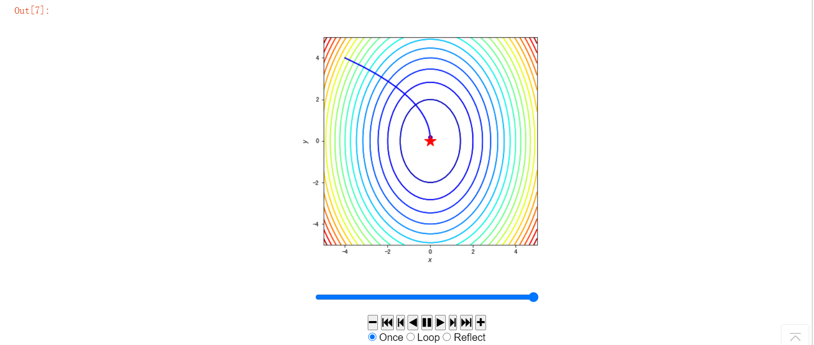
#举个例子来讲梯度下降的求解路径可视化
best_x_gd, path_list_gd = gradient_descent(f1,f1_grad,[-4.0,4.0],0.1,30)
path_list_gd

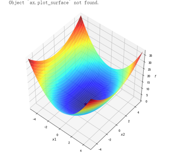
#绘制函数曲面
##先借助np.meshgrid生成网格点坐标矩阵。两个维度上每个维度显示范围为-5到5。对应网格点的函数值保存在z中
x1,x2 = np.meshgrid(np.linspace(-5.0,5.0,50), np.linspace(-5.0,5.0,50))
z = f1(x1,x2 )
minima = np.array([0, 0]) #对于函数f1,我们已知最小点为(0,0)
ax.plot_surface?
##plot_surface函数绘制3D曲面
%matplotlib inline
fig = plt.figure(figsize=(8, 8))
ax = plt.axes(projection='3d', elev=50, azim=-50)

ax.plot_surface(x1,x2, z, alpha=.8, cmap=plt.cm.jet)
ax.plot([minima[0]],[minima[1]],[f1(*minima)], 'r*', markersize=10)

ax.set_xlabel('$x1$')
ax.set_ylabel('$x2$')
ax.set_zlabel('$f$')

ax.set_xlim((-5, 5))
ax.set_ylim((-5, 5))

plt.show()
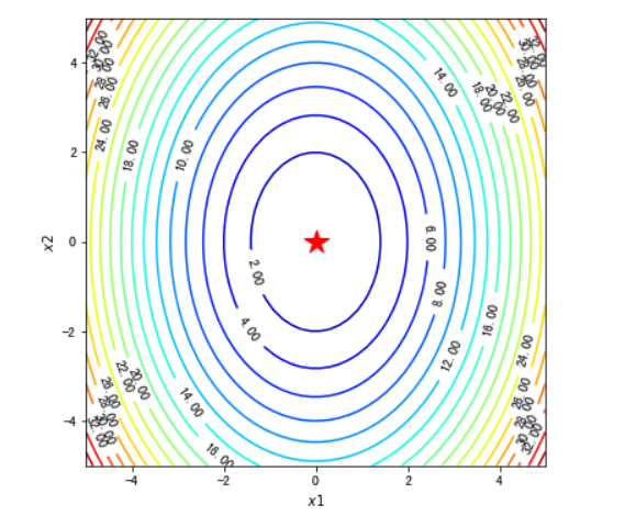
#绘制等高线和梯度场
##contour方法能够绘制等高线,clabel能够将对应线的高度(函数值)显示出来,这里我们保留两位小数(fmt='%.2f')。
dz_dx1 = elementwise_grad(f1, argnum=0)(x1, x2)
dz_dx2 = elementwise_grad(f1, argnum=1)(x1, x2)
fig, ax = plt.subplots(figsize=(6, 6))

contour = ax.contour(x1, x2, z,levels=20,cmap=plt.cm.jet)
ax.clabel(contour,fontsize=10,colors='k',fmt='%.2f')
ax.plot(*minima, 'r*', markersize=18)

ax.set_xlabel('$x1$')
ax.set_ylabel('$x2$')

ax.set_xlim((-5, 5))
ax.set_ylim((-5, 5))

plt.show()
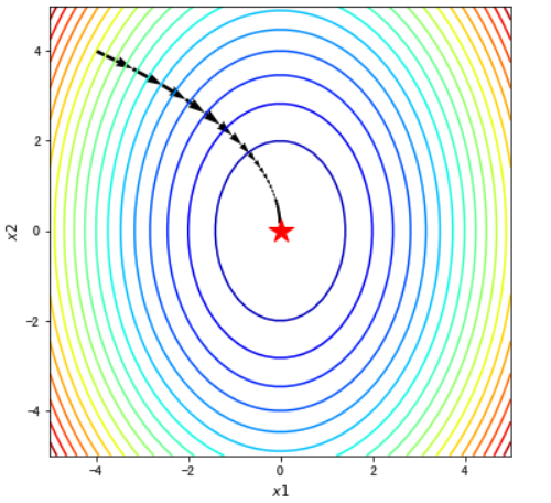
#在梯度场内使用quiver函数将路径画出来
fig, ax = plt.subplots(figsize=(6, 6))

ax.contour(x1, x2, z, levels=20,cmap=plt.cm.jet)#等高线
#绘制轨迹箭头
ax.quiver(path_list_gd[:-1,0], path_list_gd[:-1,1], path_list_gd[1:,0]-path_list_gd[:-1,0], path_list_gd[1:,1]-path_list_gd[:-1,1], scale_units='xy', angles='xy', scale=1, color='k')
#标注最优值点
ax.plot(*minima, 'r*', markersize=18)

ax.set_xlabel('$x1$')
ax.set_ylabel('$x2$')

ax.set_xlim((-5, 5))
ax.set_ylim((-5, 5))
plt.show()
#使用animation动画化
path = path_list_gd #梯度下降法的优化路径
fig, ax = plt.subplots(figsize=(6, 6))
line, = ax.plot([], [], 'b', label='Gradient Descent', lw=2) #保存路径
point, = ax.plot([], [], 'bo') #保存路径最后的点
#最开始画什么
def init_draw():
    ax.contour(x1, x2, z, levels=20, cmap=plt.cm.jet)
    ax.plot(*minima, 'r*', markersize=18) #将最小值点绘制成红色五角星
    ax.set_xlabel('$x$')
    ax.set_ylabel('$y$')
    ax.set_xlim((-5, 5))
    ax.set_ylim((-5, 5))
    return line, point
#每一步更新画什么
def update_draw(i):
    line.set_data(path[:i,0],path[:i,1])
    point.set_data(path[i-1:i,0],path[i-1:i,1])
    plt.close()
    return line, point

anim = animation.FuncAnimation(fig, update_draw, init_func=init_draw,frames=path.shape[0], interval=60, repeat_delay=5, blit=True)
HTML(anim.to_jshtml())
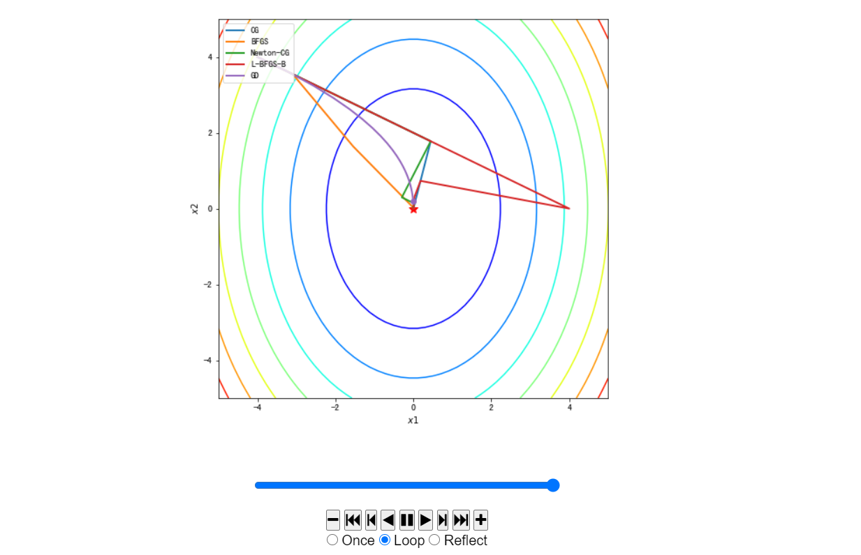
#使用scipy.optimize模块求解最优化问题。由于我们需要对优化路径进行可视化,因此minimize函数需要制定一个回调函数参数callback。
x0 = np.array([-4, 4])
def make_minimize_cb(path=[]):

    def minimize_cb(xk):
        path.append(np.copy(xk))

    return minimize_cb
#一些常见的优化方法
methods = [ "CG", "BFGS","Newton-CG","L-BFGS-B"]
#每一个方法调用minimize
import warnings
warnings.filterwarnings('ignore') #该行代码的作用是隐藏警告信息
x0 = [-4.0,4.0]
paths = []
zpaths = []
for method in methods:
    path = [x0]
    #回调函数make_minimize_cb
    res = minimize(fun=f1_grad, x0=x0,jac=True,method = method,callback=make_minimize_cb(path), bounds=[(-5, 5), (-5, 5)], tol=1e-20)
    paths.append(np.array(path))
#把刚刚自己写的梯度下降法也加进去
methods.append("GD")
paths.append(path_list_gd)
zpaths = [f1(path[:,0],path[:,1]) for path in paths]
#封装一个TrajectoryAnimation类 ,将不同算法得到的优化路径进行动画演示。
##该代码来自网址:http://louistiao.me/notes/visualizing-and-animating-optimization-algorithms-with-matplotlib/
class TrajectoryAnimation(animation.FuncAnimation):

    def __init__(self, paths, labels=[], fig=None, ax=None, frames=None,
                 interval=60, repeat_delay=5, blit=True, **kwargs):
        #如果传入的fig和ax参数为空,则新建一个fig对象和ax对象
        if fig is None:
            if ax is None:
                fig, ax = plt.subplots()
            else:
                fig = ax.get_figure()
        else:
            if ax is None:
                ax = fig.gca()
        self.fig = fig
        self.ax = ax
        self.paths = paths
        #动画的帧数等于最长的路径长度
        if frames is None:
            frames = max(path.shape[0] for path in paths) #获取最长的路径长度
        self.lines = [ax.plot([], [], label=label, lw=2)[0]
                      for _, label in zip_longest(paths, labels)]
        self.points = [ax.plot([], [], 'o', color=line.get_color())[0]
                       for line in self.lines]
        super(TrajectoryAnimation, self).__init__(fig, self.animate, init_func=self.init_anim,
                                                  frames=frames, interval=interval, blit=blit,
                                                  repeat_delay=repeat_delay, **kwargs)
    def init_anim(self):
        for line, point in zip(self.lines, self.points):
            line.set_data([], [])
            point.set_data([], [])
        return self.lines + self.points

    def animate(self, i):
        for line, point, path in zip(self.lines, self.points, self.paths):
            line.set_data(path[:i,0],path[:i,1])
            point.set_data(path[i-1:i,0],path[i-1:i,1])
            plt.close()
        return self.lines + self.points
#最后动画化对比
fig, ax = plt.subplots(figsize=(8, 8))

ax.contour(x1, x2, z, cmap=plt.cm.jet)
ax.plot(*minima, 'r*', markersize=10)

ax.set_xlabel('$x1$')
ax.set_ylabel('$x2$')

ax.set_xlim((-5, 5))
ax.set_ylim((-5, 5))

anim = TrajectoryAnimation(paths, labels=methods, ax=ax)

ax.legend(loc='upper left')
HTML(anim.to_jshtml())
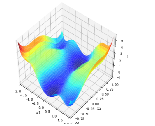
#3D可视化
##这是一个有多个局部最小值和鞍点的函数
f2 = lambda x1, x2 :((4 - 2.1*x1**2 + x1**4 / 3.) * x1**2 + x1 * x2  + (-4 + 4*x2**2) * x2 **2)
f2_grad = value_and_grad(lambda args: f2(*args))

x1,x2 = np.meshgrid(np.linspace(-2.0,2.0,50), np.linspace(-1.0,1.0,50))
z = f2(x1,x2 )
#inline改成notebook可以设置动态查看,平台内运行白屏,原因未知
%matplotlib inline
fig = plt.figure(figsize=(6, 6))
ax = plt.axes(projection='3d', elev=50, azim=-50)

ax.plot_surface(x1,x2, z, alpha=.8, cmap=plt.cm.jet)

ax.set_xlabel('$x1$')
ax.set_ylabel('$x2$')
ax.set_zlabel('$f$')

ax.set_xlim((-2.0, 2.0))
ax.set_ylim((-1.0, 1.0))

plt.show()
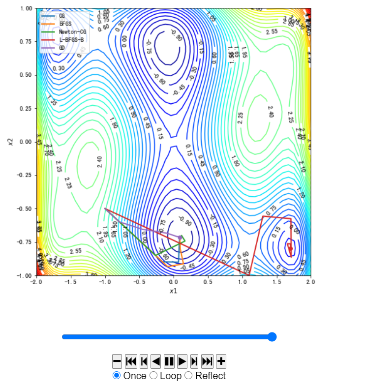
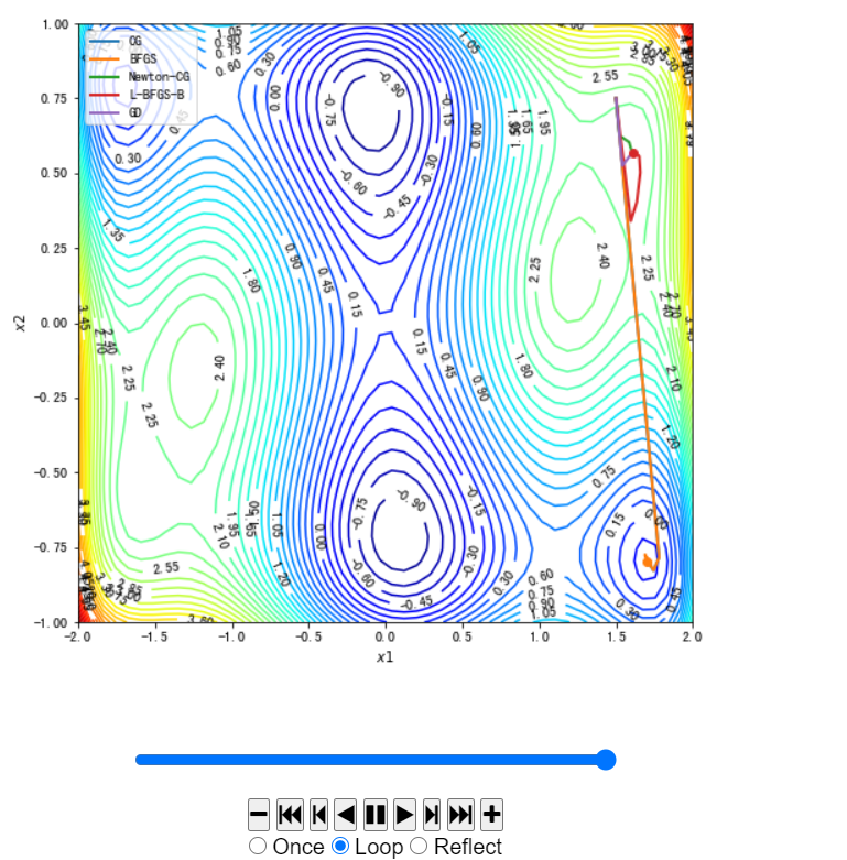
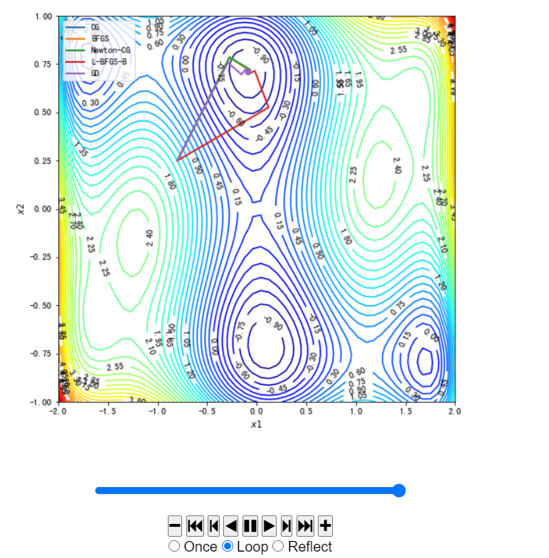
#使用Scipy中实现的不同的优化方法以及我们在本案例实现的梯度下降法进行求解。
x02 = [-1.0,-0.5]  #初始点,尝试不同初始点,[-1.0,-0.5] ,[1.5,0.75],[-0.8,0.25]
_, path_list_gd2 = gradient_descent(f2,f2_grad,x02,0.1,30) #使用梯度下降法求解

paths = []
zpaths = []
#不同方法
methods = [ "CG", "BFGS","Newton-CG","L-BFGS-B"]
for method in methods:
    path = [x02]
    res = minimize(fun=f2_grad, x0=x02,jac=True,method = method,callback=make_minimize_cb(path), bounds=[(-2.0, 2.0), (-1.0, 1.0)], tol=1e-20)
    paths.append(np.array(path))
#增加自己写的梯度下降方法
methods.append("GD")
paths.append(path_list_gd2)
zpaths = [f2(path[:,0],path[:,1]) for path in paths]
#动画形式展示
%matplotlib inline
fig, ax = plt.subplots(figsize=(8, 8))

contour = ax.contour(x1, x2, z, levels=50, cmap=plt.cm.jet)
ax.clabel(contour,fontsize=10,colors='k',fmt='%.2f')
ax.set_xlabel('$x1$')
ax.set_ylabel('$x2$')

ax.set_xlim((-2.0, 2.0))
ax.set_ylim((-1.0, 1.0))

anim = TrajectoryAnimation(paths, labels=methods, ax=ax)
ax.legend(loc='upper left')
HTML(anim.to_jshtml())
这里初始点不同图示不同,代码内不作修改,仅给出各个初始点的图像:
[-1.0, -0.5]
[1.5, 0.75]
[-0.8, 0.25]
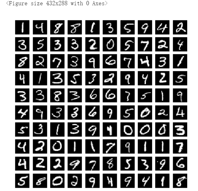
使用MNIST数据集进行算法运用:
#加载MNIST数据集
import numpy as np
f = np.load("input/mnist.npz")
X_train, y_train, X_test, y_test = f['x_train'], f['y_train'],f['x_test'], f['y_test']
f.close()
x_train = X_train.reshape((-1, 28*28)) / 255.0
x_test = X_test.reshape((-1, 28*28)) / 255.0
#随机打印一些数字
rndperm = np.random.permutation(len(x_train))
%matplotlib inline
import matplotlib.pyplot as plt
plt.gray()
fig = plt.figure( figsize=(8,8) )
for i in range(0,100):
    ax = fig.add_subplot(10,10,i+1)
    ax.matshow(x_train[rndperm[i]].reshape((28,28)))
    plt.box(False) #去掉边框
    plt.axis("off")#不显示坐标轴
plt.show()
#One-Hot编码
import pandas as pd
y_train_onehot = pd.get_dummies(y_train)
y_train_onehot.head()

我们要使用TensorFlow进行神经网络的搭建,要搭建的神经网络如图所示:
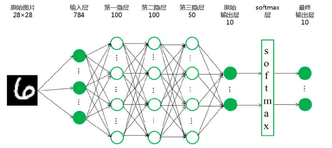
#构建手写数字识别神经网络
import tensorflow as tf
import tensorflow.keras.layers as layers
#构建并打印模型
inputs = layers.Input(shape=(28*28,), name='inputs')
#激活函数前三层设置为relu,最后一层为softmax
hidden1 = layers.Dense(100, activation='relu', name='hidden1')(inputs)
hidden2 = layers.Dense(100, activation='relu', name='hidden2')(hidden1)
hidden3 = layers.Dense(50, activation='relu', name='hidden3')(hidden2)
outputs = layers.Dense(10, activation='softmax', name='outputs')(hidden3)
deep_networks = tf.keras.Model(inputs,outputs)
deep_networks.summary()

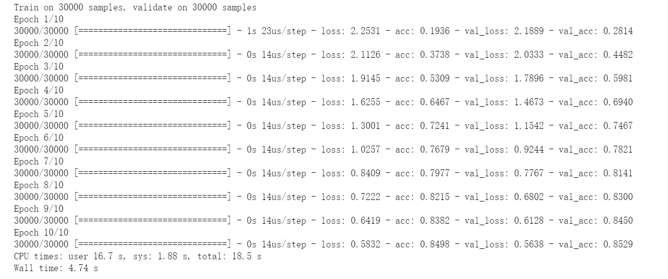
#损失函数categorical_crossentropy,优化方法SGD
##优化方法(optimizer)还可定义为RMSprop,Adam,Adagrad,Nadam
deep_networks.compile(optimizer='SGD',loss='categorical_crossentropy',metrics=['accuracy'])
###训练10次,verbose=1显示训练过程
%time history = deep_networks.fit(x_train, y_train_onehot, batch_size=500, epochs=10,validation_split=0.5,verbose=1)
#打印误差变化曲线
fig, ax = plt.subplots(figsize=(20, 8))

ax.plot(history.epoch, history.history["loss"])

ax.set_xlabel('$epoch$')
ax.set_ylabel('$loss$')

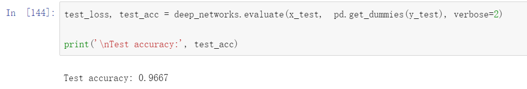
#测试并打印准确率
test_loss, test_acc = deep_networks.evaluate(x_test,  pd.get_dummies(y_test), verbose=2)

print('
Test accuracy:', test_acc)
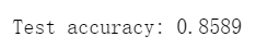
样例中给的准确率是:
这个是因为每次训练都会存在误差,属于正常现象。