这一节使用TensorFlow中的函数搭建一个简单的RNN网络,使用一串随机的模拟数据作为原始信号,让RNN网络来拟合其对应的回声信号。
样本数据为一串随机的由0,1组成的数字,将其当成发射出去的一串信号。当碰到阻挡被反弹回来时,会收到原始信号的回声。
如果步长为3,那么输入和输出的序列如下图所示:
| 原序列 | 0 | 1 | 1 | 0 | 1 | 0 | 1 | 1 | 0 | 0 | 1 | 1 | 0 | 1 | 1 |
| 回声序列 | null | null | null | 0 | 1 | 1 | 0 | 1 | 0 | 1 | 1 | 0 | 0 | 1 | 1 |
如上表所示,回声序列的前三项是null,原序列的第一个信号为0,对应的是回声序列的第四项,即回声序列的每一个数都比原序列滞后3个时序。本例的任务就是把序列截取出来,对于每个原序列来预测它的回声序列。。
构建的网络结构如下图所示:

上图中,初始的输入有5个,xt个为t时刻输入序列值,另外4个为t-1时刻隐藏层的输出值ht-1。通过一层具有4个节点的RNN网络,再接一个全连接输出两个类别,分别表示输出0,和1类别的概率。这样每个序列都会有一个对应的预测分类值,最终将整个序列生成了预测序列。
下面我们会演示一个例子,这里随机生成一个具有50000个序列样本数据,然后根据原序列生成50000个回声序列样本数据。我们每个训练截取15个序列作为一个样本,我们设置小批量大小batch_size为5。
- 我们把50000个序列,转换为5x10000的数组。
- 对数组的每一行按长度为15进行分割,每一个小批量含有5x15个序列。
- 针对每一小批量的序列,我们使用RNN网络开始迭代,迭代每一个批次中的每一组序列(5x1)。
注意这里面的5就是我们设置的batch_size大小,这和我们之前在CNN以及DNN网络中的batch_size是一样的,即一次训练使用batch_size个样本。
下面是一个小批量的原序列数据和回声序列数据,这里回声序列的前三个序列值是无效的,这主要是与我们原序列切割方式有关的。

一 定义参数并生成样本数据
np.random.seed(0)
'''
一 定义参数生成样本数据
'''

num_epochs = 5                   #迭代轮数
total_series_length = 50000      #序列样本数据长度
truncated_backprop_length = 15   #测试时截取数据长度
state_size = 4                   #中间状态长度
num_classes = 2                  #输出类别个数
echo_step =  3                   #回声步长
batch_size = 5                   #小批量大小
learning_rate = 0.4              #学习率
num_batches =total_series_length//batch_size//truncated_backprop_length   #计算一轮可以分为多少批

def generate_date():
    '''
    生成原序列和回声序列数据,回声序列滞后原序列echo_step个步长

    返回原序列和回声序列组成的元组
    '''
    #生成原序列样本数据  random.choice()随机选取内容从0和1中选取total_series_length个数据,0,1数据的概率都是0.5
    x = np.array(np.random.choice(2,total_series_length,p=[0.5,0.5]))
    #向右循环移位  如11110000->00011110
    y =np.roll(x,echo_step)
    #回声序列,前echo_step个数据清0
    y[0:echo_step] = 0

    x = x.reshape((batch_size,-1))    #5x10000
    #print(x)
    y = y.reshape((batch_size,-1))    #5x10000
    #print(y)
    return (x,y)
二 定义占位符处理输入数据
定义三个占位符,batch_x为原始序列,batch_y为回声序列真实值,init_state为循环节点的初始值。batch_x是逐个输入网络的,所以需要将输进去的数据打散,按照时间序列变成15个数组,每个数组有batch_size个元素,进行统一批处理。
'''
二 定义占位符处理输入数据
'''
batch_x = tf.placeholder(dtype=tf.float32,shape=[batch_size,truncated_backprop_length])    #原始序列
batch_y = tf.placeholder(dtype=tf.int32,shape=[batch_size,truncated_backprop_length])      #回声序列 作为标签
init_state = tf.placeholder(dtype=tf.float32,shape=[batch_size,state_size])                #循环节点的初始状态值


#将batch_x沿axis = 1(列)的轴进行拆分    返回一个list 每个元素都是一个数组   [(5,),(5,)....] 一共15个元素,即15个序列
inputs_series = tf.unstack(batch_x,axis=1)
labels_series = tf.unstack(batch_y,axis=1)
三 定义网络结构
定义一层循环与一层全网络连接。由于数据是一个二维数组序列,所以需要通过循环将输入数据按照原有序列逐个输入网络,并输出对应的predictions序列,同样的,对于每个序列值都要对其做loss计算,在loss计算使用了spare_softmax_cross_entropy_with_logits函数,因为label的最大值正好是1,而且是一位的,就不需要在使用one_hot编码了,最终将所有的loss均值放入优化器中。
'''
三 定义RNN网络结构

一个输入样本由15个输入序列组成 一个小批量包含5个输入样本
'''
current_state = init_state     #存放当前的状态
predictions_series = []        #存放一个小批量中每个输入样本的预测序列值 每个元素为5x2 共有15个元素
losses = []                    #存放一个小批量中每个输入样本训练的损失值 每个元素是一个标量,共有15个元素

#使用一个循环,按照序列逐个输入
for current_input,labels in zip(inputs_series,labels_series):
    #确定形状为batch_size x 1
    current_input = tf.reshape(current_input,[batch_size,1])
    '''
       加入初始状态
       5 x 1序列值和 5 x 4中间状态 按列连接,得到 5 x 5数组 构成输入数据
    '''
    input_and_state_concatenated = tf.concat([current_input,current_state],1)
    #隐藏层激活函数选择tanh 5x4
    next_state = tf.contrib.layers.fully_connected(input_and_state_concatenated,state_size,activation_fn = tf.tanh)
    current_state = next_state
    #输出层 激活函数选择None,即直接输出 5x2
    logits = tf.contrib.layers.fully_connected(next_state,num_classes,activation_fn = None)
    #计算代价
    loss = tf.reduce_mean(tf.nn.sparse_softmax_cross_entropy_with_logits(labels=labels,logits = logits))
    losses.append(loss)
    #经过softmax计算预测值 5x2  注意这里并不是标签值 这里是one_hot编码
    predictions =  tf.nn.softmax(logits)
    predictions_series.append(predictions)

total_loss = tf.reduce_mean(losses)
train_step = tf.train.AdagradOptimizer(learning_rate).minimize(total_loss)
四 建立session训练数据并可视化输出
建立session,初始化RNN循环节点的值为0。总样本迭代5轮,每一轮迭代完调用plot函数生成图像。
'''
四 建立session训练数据
'''
with tf.Session() as sess:
    sess.run(tf.global_variables_initializer())
    loss_list = []            #list 存放每一小批量的代价值

    #开始迭代每一轮
    for epoch_idx in range(num_epochs):
        #生成原序列和回声序列数据
        x,y = generate_date()

        #初始化循环节点状态值
        _current_state = np.zeros((batch_size,state_size))

        print('New date,epoch',epoch_idx)

        #迭代每一小批量
        for batch_idx in range(num_batches):
            #计算当前batch的起始索引
            start_idx = batch_idx * truncated_backprop_length
            #计算当前batch的结束索引
            end_idx = start_idx + truncated_backprop_length

            #当前批次的原序列值
            batchx = x[:,start_idx:end_idx]
            #当前批次的回声序列值
            batchy = y[:,start_idx:end_idx]

            #开始训练当前批次样本
            _total_loss,_train_step,_current_state,_predictions_series = sess.run(
                    [total_loss,train_step,current_state,predictions_series],
                    feed_dict = {
                            batch_x:batchx,
                            batch_y:batchy,
                            init_state:_current_state
                            })

            loss_list.append(_total_loss)

            if batch_idx % 100 == 0:
                print('Step {0} Loss {1}'.format(batch_idx,_total_loss))
        #可视化输出
        plot(loss_list,_predictions_series,batchx,batchy)
        #print(batchx)
        #print(batchy)
def plot(loss_list, predictions_series, batchx, batchy):
    '''
    绘制一个小批量中每一个原序列样本,回声序列样本,预测序列样本图像

    args:
        loss_list:list 存放每一个批次训练的代价值
        predictions_series:list长度为5  存放一个批次中每个输入序列的预测序列值 注意这里每个元素(5x2)都是one_hot编码
        batchx:当前批次的原序列 5x15
        batchy:当前批次的回声序列 5x15
    '''
    plt.figure(figsize=(3.2*3,2.4*2))
    #创建子图 2行3列选择第一个  绘制代价值
    plt.subplot(2, 3, 1)
    plt.cla()
    plt.plot(loss_list)


    #迭代每一个序列  循环5次
    for batch_series_idx in range(batch_size):
        #获取第batch_series_idx个序列的预测值(one_hot编码) 15x2
        one_hot_output_series = np.array(predictions_series)[:, batch_series_idx, :]
        #转换为标签值 (15,)
        single_output_series = np.array([(1 if out[0] < 0.5 else 0) for out in one_hot_output_series])


        #绘制第batch_series_idx + 2个子图
        plt.subplot(2, 3, batch_series_idx + 2)
        plt.cla()
        #设置x轴 y轴坐标值范围
        plt.axis([0, truncated_backprop_length, 0, 2])
        #获取原序列x坐标值
        left_offset = range(truncated_backprop_length)
        #获取回声序列x坐标值 滞后3个步长
        left_offset2 = range(echo_step,truncated_backprop_length + echo_step)

        label1 = "past values"
        label2 = "True echo values"
        label3 = "Predictions"
        #绘制原序列
        plt.plot(left_offset2, batchx[batch_series_idx, :]*0.2+1.5, "o--b", label=label1)
        #绘制真实回声序列
        plt.plot(left_offset, batchy[batch_series_idx, :]*0.2+0.8,"x--b", label=label2)
        #绘制预测回声序列
        plt.plot(left_offset,  single_output_series*0.2+0.1 , "o--r", label=label3)

    plt.legend(loc='best')
    plt.show()
函数中将输入的原序列,回声序列和预测的序列同时输出在图像中。按照小批量样本的个数生成图像。为了让三个序列看起来更明显,将其缩放0.2,并且调节每个图像的高度。同时将原始序列在显示中滞后echo_step个序列,将三个图像放在同一序列顺序比较。
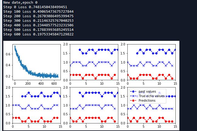
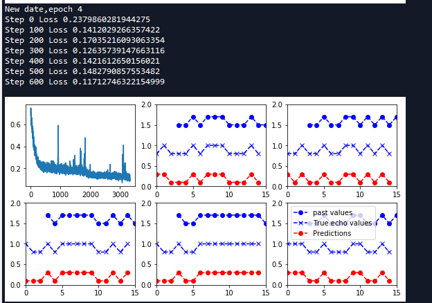
如上图,最下面的是预测的序列,中间的为回声序列,从图像上可以看出预测序列和回声序列几乎相同,表明RNN网络已经完全可以学习到回声的规则。
完整代码:


# -*- coding: utf-8 -*-
"""
Created on Tue May  8 08:45:40 2018

@author: zy
"""

'''
使用RNN网络拟合回声信号序列

使用一串随机的模拟数据作为原始信号,让RNN网络来拟合其对应的回声信号
样本数据为一串随机的由0,1组成的数字,将其当成发射出去的一串信号。当碰到阻挡被反弹回来时,会收到原始信号的回音

如果步长为3,那么输入和输出的序列序列如下:
原序列     0   1    1   |   0   1    0   .....     1
回声序列 null null null |   0   1    1   .....     0
'''

import tensorflow  as tf
import numpy as np
import matplotlib.pyplot as plt

np.random.seed(0)
'''
一 定义参数生成样本数据
'''

num_epochs = 5                   #迭代轮数
total_series_length = 50000      #序列样本数据长度
truncated_backprop_length = 15   #测试时截取数据长度
state_size = 4                   #中间状态长度
num_classes = 2                  #输出类别个数
echo_step =  3                   #回声步长
batch_size = 5                   #小批量大小
learning_rate = 0.4              #学习率
num_batches =total_series_length//batch_size//truncated_backprop_length   #计算一轮可以分为多少批

def generate_date():
    '''
    生成原序列和回声序列数据,回声序列滞后原序列echo_step个步长

    返回原序列和回声序列组成的元组
    '''
    #生成原序列样本数据  random.choice()随机选取内容从0和1中选取total_series_length个数据,0,1数据的概率都是0.5
    x = np.array(np.random.choice(2,total_series_length,p=[0.5,0.5]))
    #向右循环移位  如11110000->00011110
    y =np.roll(x,echo_step)
    #回声序列,前echo_step个数据清0
    y[0:echo_step] = 0

    x = x.reshape((batch_size,-1))    #5x10000
    #print(x)
    y = y.reshape((batch_size,-1))    #5x10000
    #print(y)
    return (x,y)


'''
二 定义占位符处理输入数据
'''
batch_x = tf.placeholder(dtype=tf.float32,shape=[batch_size,truncated_backprop_length])    #原始序列
batch_y = tf.placeholder(dtype=tf.int32,shape=[batch_size,truncated_backprop_length])      #回声序列 作为标签
init_state = tf.placeholder(dtype=tf.float32,shape=[batch_size,state_size])                #循环节点的初始状态值


#将batch_x沿axis = 1(列)的轴进行拆分    返回一个list 每个元素都是一个数组   [(5,),(5,)....] 一共15个元素,即15个序列
inputs_series = tf.unstack(batch_x,axis=1)
labels_series = tf.unstack(batch_y,axis=1)


'''
三 定义RNN网络结构

一个输入样本由15个输入序列组成 一个小批量包含5个输入样本
'''
current_state = init_state     #存放当前的状态
predictions_series = []        #存放一个小批量中每个输入样本的预测序列值 每个元素为5x2 共有15个元素
losses = []                    #存放一个小批量中每个输入样本训练的损失值 每个元素是一个标量,共有15个元素

#使用一个循环,按照序列逐个输入
for current_input,labels in zip(inputs_series,labels_series):
    #确定形状为batch_size x 1
    current_input = tf.reshape(current_input,[batch_size,1])
    '''
       加入初始状态
       5 x 1序列值和 5 x 4中间状态 按列连接,得到 5 x 5数组 构成输入数据
    '''
    input_and_state_concatenated = tf.concat([current_input,current_state],1)
    #隐藏层激活函数选择tanh 5x4
    next_state = tf.contrib.layers.fully_connected(input_and_state_concatenated,state_size,activation_fn = tf.tanh)
    current_state = next_state
    #输出层 激活函数选择None,即直接输出 5x2
    logits = tf.contrib.layers.fully_connected(next_state,num_classes,activation_fn = None)
    #计算代价
    loss = tf.reduce_mean(tf.nn.sparse_softmax_cross_entropy_with_logits(labels=labels,logits = logits))
    losses.append(loss)
    #经过softmax计算预测值 5x2  注意这里并不是标签值 这里是one_hot编码
    predictions =  tf.nn.softmax(logits)

    predictions_series.append(predictions)


total_loss = tf.reduce_mean(losses)
train_step = tf.train.AdagradOptimizer(learning_rate).minimize(total_loss)


def plot(loss_list, predictions_series, batchx, batchy):
    '''
    绘制一个小批量中每一个原序列样本,回声序列样本,预测序列样本图像

    args:
        loss_list:list 存放每一个批次训练的代价值
        predictions_series:list长度为5  存放一个批次中每个输入序列的预测序列值 注意这里每个元素(5x2)都是one_hot编码
        batchx:当前批次的原序列 5x15
        batchy:当前批次的回声序列 5x15
    '''
    plt.figure(figsize=(3.2*3,2.4*2))
    #创建子图 2行3列选择第一个  绘制代价值
    plt.subplot(2, 3, 1)
    plt.cla()
    plt.plot(loss_list)


    #迭代每一个序列  循环5次
    for batch_series_idx in range(batch_size):
        #获取第batch_series_idx个序列的预测值(one_hot编码) 15x2
        one_hot_output_series = np.array(predictions_series)[:, batch_series_idx, :]
        #转换为标签值 (15,)
        single_output_series = np.array([(1 if out[0] < 0.5 else 0) for out in one_hot_output_series])


        #绘制第batch_series_idx + 2个子图
        plt.subplot(2, 3, batch_series_idx + 2)
        plt.cla()
        #设置x轴 y轴坐标值范围
        plt.axis([0, truncated_backprop_length, 0, 2])
        #获取原序列x坐标值
        left_offset = range(truncated_backprop_length)
        #获取回声序列x坐标值 滞后3个步长
        left_offset2 = range(echo_step,truncated_backprop_length + echo_step)

        label1 = "past values"
        label2 = "True echo values"
        label3 = "Predictions"
        #绘制原序列
        plt.plot(left_offset2, batchx[batch_series_idx, :]*0.2+1.5, "o--b", label=label1)
        #绘制真实回声序列
        plt.plot(left_offset, batchy[batch_series_idx, :]*0.2+0.8,"x--b", label=label2)
        #绘制预测回声序列
        plt.plot(left_offset,  single_output_series*0.2+0.1 , "o--r", label=label3)

    plt.legend(loc='best')
    plt.show()

'''
四 建立session训练数据
'''
with tf.Session() as sess:
    sess.run(tf.global_variables_initializer())
    loss_list = []            #list 存放每一小批量的代价值

    #开始迭代每一轮
    for epoch_idx in range(num_epochs):
        #生成原序列和回声序列数据
        x,y = generate_date()

        #初始化循环节点状态值
        _current_state = np.zeros((batch_size,state_size))

        print('New date,epoch',epoch_idx)

        #迭代每一小批量
        for batch_idx in range(num_batches):
            #计算当前batch的起始索引
            start_idx = batch_idx * truncated_backprop_length
            #计算当前batch的结束索引
            end_idx = start_idx + truncated_backprop_length

            #当前批次的原序列值
            batchx = x[:,start_idx:end_idx]
            #当前批次的回声序列值
            batchy = y[:,start_idx:end_idx]

            #开始训练当前批次样本
            _total_loss,_train_step,_current_state,_predictions_series = sess.run(
                    [total_loss,train_step,current_state,predictions_series],
                    feed_dict = {
                            batch_x:batchx,
                            batch_y:batchy,
                            init_state:_current_state
                            })

            loss_list.append(_total_loss)

            if batch_idx % 100 == 0:
                print('Step {0} Loss {1}'.format(batch_idx,_total_loss))
        #可视化输出
        plot(loss_list,_predictions_series,batchx,batchy)
        #print(batchx)
        #print(batchy)