在使用卷积神经网络时,我们也总结了一些训练技巧,下面就来介绍如何对卷积核进行优化,以及多通道卷积技术的使用。
一 优化卷积核
在实际的卷积训练中,为了加快速度,常常把卷积核裁开。比如一个3x3的卷积核,可以裁成一个3x1和1x3的卷积核(通过矩阵乘法得知),分别对原有输入做卷积运算,这样可以大大提升运算的速度。
原理:在浮点运算中乘法消耗的资源比较多,我们目的就是尽量减少乘法运算。
- 比如对一个5x2的原始图片进行一次3x3的SAME卷积,相当于生成的5x2的像素中,每一个像素都需要经历3x3次乘法,那么一共是90次。
- 同样是这样图片,如果先进行一次3X1的SAME卷积,相当于生成的5x2的像素中,每一个像素都需要经历3x1次乘法,那么一共是30次。再进行一次1x3的SAME卷积也是计算30次,在一起总共60次。
这仅仅是一个很小的数据张量,而且随着张量维度的增大,层数的增多,减少的运算更多。运算量减少了,运算速度会更快。
接下来我会演示一个例子,仍然是改写第十三节对cifar10数据集分类的例子。
# -*- coding: utf-8 -*-
"""
Created on Thu May  3 12:29:16 2018

@author: zy
"""

'''
优化卷积核 提高运算速度
'''

'''
建立一个带有全局平均池化层的卷积神经网络  并对CIFAR-10数据集进行分类
1.使用3个卷积层的同卷积操作,滤波器大小为5x5,每个卷积层后面都会跟一个步长为2x2的池化层,滤波器大小为2x2
2.对输出的10个feature map进行全局平均池化,得到10个特征
3.对得到的10个特征进行softmax计算,得到分类
'''

import cifar10_input
import tensorflow as tf
import numpy as np


def weight_variable(shape):
    '''
    初始化权重

    args:
        shape:权重shape
    '''
    initial = tf.truncated_normal(shape=shape,mean=0.0,stddev=0.1)
    return tf.Variable(initial)

def bias_variable(shape):
    '''
    初始化偏置

    args:
        shape:偏置shape
    '''
    initial =tf.constant(0.1,shape=shape)
    return tf.Variable(initial)


def conv2d(x,W):
    '''
    卷积运算 ,使用SAME填充方式   卷积层后
         out_height = in_hight / strides_height(向上取整)
         out_width = in_width / strides_width(向上取整)

    args:
        x:输入图像 形状为[batch,in_height,in_width,in_channels]
        W:权重 形状为[filter_height,filter_width,in_channels,out_channels]
    '''
    return tf.nn.conv2d(x,W,strides=[1,1,1,1],padding='SAME')


def max_pool_2x2(x):
    '''
    最大池化层,滤波器大小为2x2,'SAME'填充方式  池化层后
         out_height = in_hight / strides_height(向上取整)
         out_width = in_width / strides_width(向上取整)

    args:
        x:输入图像 形状为[batch,in_height,in_width,in_channels]
    '''
    return tf.nn.max_pool(x,ksize=[1,2,2,1],strides=[1,2,2,1],padding='SAME')


def avg_pool_6x6(x):
    '''
    全局平均池化层,使用一个与原有输入同样尺寸的filter进行池化,'SAME'填充方式  池化层后
         out_height = in_hight / strides_height(向上取整)
         out_width = in_width / strides_width(向上取整)

    args;
        x:输入图像 形状为[batch,in_height,in_width,in_channels]
    '''
    return tf.nn.avg_pool(x,ksize=[1,6,6,1],strides=[1,6,6,1],padding='SAME')

def print_op_shape(t):
    '''
    输出一个操作op节点的形状

    args:
        t:必须是一个tensor类型
        t.get_shape()返回一个元组  .as_list()转换为list
    '''
    print(t.op.name,'',t.get_shape().as_list())

'''
一 引入数据集
'''
batch_size = 128
learning_rate = 1e-4
training_step = 15000
display_step = 200
#数据集目录
data_dir = './cifar10_data/cifar-10-batches-bin'
print('begin')
#获取训练集数据
images_train,labels_train = cifar10_input.inputs(eval_data=False,data_dir = data_dir,batch_size=batch_size)
print('begin data')


'''
二 定义网络结构
'''
#定义占位符
input_x = tf.placeholder(dtype=tf.float32,shape=[None,24,24,3])   #图像大小24x24x
input_y = tf.placeholder(dtype=tf.float32,shape=[None,10])        #0-9类别

x_image = tf.reshape(input_x,[batch_size,24,24,3])

#1.卷积层 ->池化层
W_conv1 = weight_variable([5,5,3,64])
b_conv1 = bias_variable([64])


h_conv1 = tf.nn.relu(conv2d(x_image,W_conv1) + b_conv1)    #输出为[-1,24,24,64]
print_op_shape(h_conv1)
h_pool1 = max_pool_2x2(h_conv1)                            #输出为[-1,12,12,64]
print_op_shape(h_pool1)


#2.卷积层 ->池化层   卷积核做优化
W_conv21 = weight_variable([5,1,64,64])
b_conv21 = bias_variable([64])


h_conv21 = tf.nn.relu(conv2d(h_pool1,W_conv21) + b_conv21)    #输出为[-1,12,12,64]
print_op_shape(h_conv21)

W_conv2 = weight_variable([1,5,64,64])
b_conv2 = bias_variable([64])


h_conv2 = tf.nn.relu(conv2d(h_conv21,W_conv2) + b_conv2)     #输出为[-1,12,12,64]
print_op_shape(h_conv2)

h_pool2 = max_pool_2x2(h_conv2)                              #输出为[-1,6,6,64]
print_op_shape(h_pool2)


#3.卷积层 ->全局平均池化层
W_conv3 = weight_variable([5,5,64,10])
b_conv3 = bias_variable([10])

h_conv3 = tf.nn.relu(conv2d(h_pool2,W_conv3) + b_conv3)   #输出为[-1,6,6,10]
print_op_shape(h_conv3)

nt_hpool3 = avg_pool_6x6(h_conv3)                         #输出为[-1,1,1,10]
print_op_shape(nt_hpool3)
nt_hpool3_flat = tf.reshape(nt_hpool3,[-1,10])

y_conv = tf.nn.softmax(nt_hpool3_flat)

'''
三 定义求解器
'''

#softmax交叉熵代价函数
cost = tf.reduce_mean(-tf.reduce_sum(input_y * tf.log(y_conv),axis=1))

#求解器
train = tf.train.AdamOptimizer(learning_rate).minimize(cost)

#返回一个准确度的数据
correct_prediction = tf.equal(tf.arg_max(y_conv,1),tf.arg_max(input_y,1))
#准确率
accuracy = tf.reduce_mean(tf.cast(correct_prediction,dtype=tf.float32))

'''
四 开始训练
'''
sess = tf.Session();
sess.run(tf.global_variables_initializer())
# 启动计算图中所有的队列线程 调用tf.train.start_queue_runners来将文件名填充到队列,否则read操作会被阻塞到文件名队列中有值为止。
tf.train.start_queue_runners(sess=sess)

for step in range(training_step):
    #获取batch_size大小数据集
    image_batch,label_batch = sess.run([images_train,labels_train])

    #one hot编码
    label_b = np.eye(10,dtype=np.float32)[label_batch]

    #开始训练
    train.run(feed_dict={input_x:image_batch,input_y:label_b},session=sess)

    if step % display_step == 0:
        train_accuracy = accuracy.eval(feed_dict={input_x:image_batch,input_y:label_b},session=sess)
        print('Step {0} tranining accuracy {1}'.format(step,train_accuracy))
运行结果如下:


二 多通道卷积技术
多通道卷积技术详细内容可以点击:第十四节,卷积神经网络之经典网络Inception(四)
多通道卷积可以理解为一种新的CNN网络模型,在原有的卷积模型基础上扩展。
- 在原有的卷积层中是使用单个尺寸的卷积核对输入数据进行卷积操作,生成若干个feature map。

- 而多通道卷积的变化就是,在单个卷积层中加入若干个不同尺寸的过滤器,这样会使生成的feature map特征更加多样性。

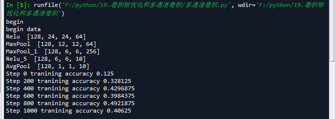
接下来我会演示一个例子,仍然是改写第十三节对cifar10数据集分类的例子,我们为网络的卷积层增加不同尺寸的卷积核。这里将原有的5x5卷积,扩展到7x7卷积,1x1卷积,3x3卷积,并将它们的输出通过tf.concat()函数并在一起。
代码如下:
# -*- coding: utf-8 -*-
"""
Created on Sat May  5 17:59:50 2018

@author: zy
"""

'''
多通道卷积技术
'''


'''
建立一个带有全局平均池化层的卷积神经网络  并对CIFAR-10数据集进行分类
1.使用3个卷积层的同卷积操作,滤波器大小为5x5,每个卷积层后面都会跟一个步长为2x2的池化层,滤波器大小为2x2
2.对输出的10个feature map进行全局平均池化,得到10个特征
3.对得到的10个特征进行softmax计算,得到分类
'''

import cifar10_input
import tensorflow as tf
import numpy as np

def weight_variable(shape):
    '''
    初始化权重

    args:
        shape:权重shape
    '''
    initial = tf.truncated_normal(shape=shape,mean=0.0,stddev=0.1)
    return tf.Variable(initial)

def bias_variable(shape):
    '''
    初始化偏置

    args:
        shape:偏置shape
    '''
    initial =tf.constant(0.1,shape=shape)
    return tf.Variable(initial)


def conv2d(x,W):
    '''
    卷积运算 ,使用SAME填充方式   卷积层后
         out_height = in_hight / strides_height(向上取整)
         out_width = in_width / strides_width(向上取整)

    args:
        x:输入图像 形状为[batch,in_height,in_width,in_channels]
        W:权重 形状为[filter_height,filter_width,in_channels,out_channels]
    '''
    return tf.nn.conv2d(x,W,strides=[1,1,1,1],padding='SAME')


def max_pool_2x2(x):
    '''
    最大池化层,滤波器大小为2x2,'SAME'填充方式  池化层后
         out_height = in_hight / strides_height(向上取整)
         out_width = in_width / strides_width(向上取整)

    args:
        x:输入图像 形状为[batch,in_height,in_width,in_channels]
    '''
    return tf.nn.max_pool(x,ksize=[1,2,2,1],strides=[1,2,2,1],padding='SAME')


def avg_pool_6x6(x):
    '''
    全局平均池化层,使用一个与原有输入同样尺寸的filter进行池化,'SAME'填充方式  池化层后
         out_height = in_hight / strides_height(向上取整)
         out_width = in_width / strides_width(向上取整)

    args;
        x:输入图像 形状为[batch,in_height,in_width,in_channels]
    '''
    return tf.nn.avg_pool(x,ksize=[1,6,6,1],strides=[1,6,6,1],padding='SAME')

def print_op_shape(t):
    '''
    输出一个操作op节点的形状

    args:
        t:必须是一个tensor类型
        t.get_shape()返回一个元组  .as_list()转换为list
    '''
    print(t.op.name,'',t.get_shape().as_list())

'''
一 引入数据集
'''
batch_size = 128
learning_rate = 1e-4
training_step = 15000
display_step = 200
#数据集目录
data_dir = './cifar10_data/cifar-10-batches-bin'
print('begin')
#获取训练集数据
images_train,labels_train = cifar10_input.inputs(eval_data=False,data_dir = data_dir,batch_size=batch_size)
print('begin data')


'''
二 定义网络结构
'''
#定义占位符
input_x = tf.placeholder(dtype=tf.float32,shape=[None,24,24,3])   #图像大小24x24x
input_y = tf.placeholder(dtype=tf.float32,shape=[None,10])        #0-9类别

x_image = tf.reshape(input_x,[batch_size,24,24,3])

#1.卷积层 ->池化层
W_conv1 = weight_variable([5,5,3,64])
b_conv1 = bias_variable([64])


h_conv1 = tf.nn.relu(conv2d(x_image,W_conv1) + b_conv1)    #输出为[-1,24,24,64]
print_op_shape(h_conv1)
h_pool1 = max_pool_2x2(h_conv1)                            #输出为[-1,12,12,64]
print_op_shape(h_pool1)


#2.卷积层 ->池化层  这里使用多通道卷积
W_conv2_1x1 = weight_variable([1,1,64,64])
b_conv2_1x1 = bias_variable([64])

W_conv2_3x3 = weight_variable([3,3,64,64])
b_conv2_3x3 = bias_variable([64])

W_conv2_5x5 = weight_variable([5,5,64,64])
b_conv2_5x5 = bias_variable([64])

W_conv2_7x7 = weight_variable([7,7,64,64])
b_conv2_7x7 = bias_variable([64])


h_conv2_1x1 = tf.nn.relu(conv2d(h_pool1,W_conv2_1x1) + b_conv2_1x1)    #输出为[-1,12,12,64]
h_conv2_3x3 = tf.nn.relu(conv2d(h_pool1,W_conv2_3x3) + b_conv2_3x3)    #输出为[-1,12,12,64]
h_conv2_5x5 = tf.nn.relu(conv2d(h_pool1,W_conv2_5x5) + b_conv2_5x5)    #输出为[-1,12,12,64]
h_conv2_7x7 = tf.nn.relu(conv2d(h_pool1,W_conv2_7x7) + b_conv2_7x7)    #输出为[-1,12,12,64]

#合并 3表示沿着通道合并
h_conv2  = tf.concat((h_conv2_1x1,h_conv2_3x3,h_conv2_5x5,h_conv2_7x7),axis=3)  #输出为[-1,12,12,256]

h_pool2 = max_pool_2x2(h_conv2)                            #输出为[-1,6,6,256]
print_op_shape(h_pool2)


#3.卷积层 ->全局平均池化层
W_conv3 = weight_variable([5,5,256,10])
b_conv3 = bias_variable([10])

h_conv3 = tf.nn.relu(conv2d(h_pool2,W_conv3) + b_conv3)   #输出为[-1,6,6,10]
print_op_shape(h_conv3)

nt_hpool3 = avg_pool_6x6(h_conv3)                         #输出为[-1,1,1,10]
print_op_shape(nt_hpool3)
nt_hpool3_flat = tf.reshape(nt_hpool3,[-1,10])

y_conv = tf.nn.softmax(nt_hpool3_flat)

'''
三 定义求解器
'''

#softmax交叉熵代价函数
cost = tf.reduce_mean(-tf.reduce_sum(input_y * tf.log(y_conv),axis=1))

#求解器
train = tf.train.AdamOptimizer(learning_rate).minimize(cost)

#返回一个准确度的数据
correct_prediction = tf.equal(tf.arg_max(y_conv,1),tf.arg_max(input_y,1))
#准确率
accuracy = tf.reduce_mean(tf.cast(correct_prediction,dtype=tf.float32))

'''
四 开始训练
'''
sess = tf.Session();
sess.run(tf.global_variables_initializer())
# 启动计算图中所有的队列线程 调用tf.train.start_queue_runners来将文件名填充到队列,否则read操作会被阻塞到文件名队列中有值为止。
tf.train.start_queue_runners(sess=sess)

for step in range(training_step):
    #获取batch_size大小数据集
    image_batch,label_batch = sess.run([images_train,labels_train])

    #one hot编码
    label_b = np.eye(10,dtype=np.float32)[label_batch]

    #开始训练
    train.run(feed_dict={input_x:image_batch,input_y:label_b},session=sess)

    if step % display_step == 0:
        train_accuracy = accuracy.eval(feed_dict={input_x:image_batch,input_y:label_b},session=sess)
        print('Step {0} tranining accuracy {1}'.format(step,train_accuracy))
运行结果如下(我只截取了一部分):