最先提出是这篇论文:https://dl.acm.org/doi/10.5555/2503308.2188410
用于判断两个分布p和q是否相同。
基本假设:如果两个分布生成足够多的样本在f上对应的均值都相等,那么可以认为这两个分布是同一个分布。
基本两个分布的样本,通过寻找在样本空间上的连续函数f,求不用分布的样本在f上的函数值的均值,通过把两个均值做差可以得到两个分布对应于f的mean discrepancy。寻找一个f,使得这个mean discrepancy有最大值。这个最大值就是MMD。取MMD作为检验统计量,如果这个值足够的小,则认为两个分布相同。否则认为它们不相同。
定义如下:

MMD的经验估计如下。x,y分别是从p和q通过独立同分布采样得到的两个数据集。

在给定两个分布的观测集X,Y的情况下,这个结果会严重依赖于给定的函数集F。为了能表示MMD的性质:当且仅当p和q是相同分布的时候MMD为0,那么要求F足够rich;另一方面为了使检验具有足够的连续性(be consistent in power),从而使得MMD的经验估计可以随着观测集规模增大迅速收敛到它的期望,F必须足够restrictive。文中证明了当F是universal RKHS上的(unit ball)单位球时,可以满足上面两个性质。


上界就是f:be a unit ball in a universal RKHS,比如高斯核或者拉普拉斯核。进一步给定RKHS对应合函数,则MMD的平方可以表示为:

估计如下:


补充:


如何得到。参看知乎https://zhuanlan.zhihu.com/p/1142648310 和 http://iera.name/a-story-of-basis-and-kernel-part-ii-reproducing-kernel-hilbert-space/
代码参考https://github.com/easezyc/deep-transfer-learning/blob/5e94d519b7bb7f94f0e43687aa4663aca18357de/MUDA/MFSAN/MFSAN_3src/mmd.py
import torch
def guassian_kernel(source, target, kernel_mul=2.0, kernel_num=5, fix_sigma=None):
'''
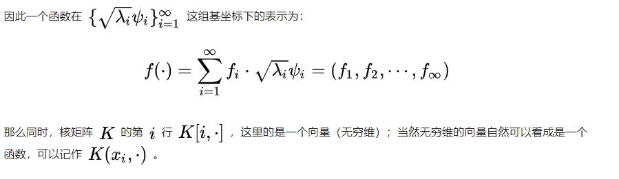
将源域数据和目标域数据转化为核矩阵,即上文中的K
Params:
source: 源域数据,行表示样本数目,列表示样本数据维度
target: 目标域数据 同source
kernel_mul: 多核MMD,以bandwidth为中心,两边扩展的基数,比如bandwidth/kernel_mul, bandwidth, bandwidth*kernel_mul
kernel_num: 取不同高斯核的数量
fix_sigma: 是否固定,如果固定,则为单核MMD
Return:
sum(kernel_val): 多个核矩阵之和
'''
n_samples = int(source.size()[0])+int(target.size()[0])
# 求矩阵的行数,即两个域的的样本总数,一般source和target的尺度是一样的,这样便于计算
total = torch.cat([source, target], dim=0)#将source,target按列方向合并
#将total复制(n+m)份
total0 = total.unsqueeze(0).expand(int(total.size(0)), int(total.size(0)), int(total.size(1)))
#将total的每一行都复制成(n+m)行,即每个数据都扩展成(n+m)份
total1 = total.unsqueeze(1).expand(int(total.size(0)), int(total.size(0)), int(total.size(1)))
# total1 - total2 得到的矩阵中坐标(i,j, :)代表total中第i行数据和第j行数据之间的差
# sum函数,对第三维进行求和,即平方后再求和,获得高斯核指数部分的分子,是L2范数的平方
L2_distance_square = ((total0-total1)**2).sum(2)
#调整高斯核函数的sigma值
if fix_sigma:
bandwidth = fix_sigma
else:
bandwidth = torch.sum(L2_distance_square) / (n_samples**2-n_samples)
# 多核MMD
#以fix_sigma为中值,以kernel_mul为倍数取kernel_num个bandwidth值(比如fix_sigma为1时,得到[0.25,0.5,1,2,4]
bandwidth /= kernel_mul ** (kernel_num // 2)
bandwidth_list = [bandwidth * (kernel_mul**i) for i in range(kernel_num)]
print(bandwidth_list)
#高斯核函数的数学表达式
kernel_val = [torch.exp(-L2_distance_square / bandwidth_temp) for bandwidth_temp in bandwidth_list]
#得到最终的核矩阵
return sum(kernel_val)#/len(kernel_val)
def mmd_rbf(source, target, kernel_mul=2.0, kernel_num=5, fix_sigma=None):
'''
计算源域数据和目标域数据的MMD距离
Params:
source: 源域数据,行表示样本数目,列表示样本数据维度
target: 目标域数据 同source
kernel_mul: 多核MMD,以bandwidth为中心,两边扩展的基数,比如bandwidth/kernel_mul, bandwidth, bandwidth*kernel_mul
kernel_num: 取不同高斯核的数量
fix_sigma: 是否固定,如果固定,则为单核MMD
Return:
loss: MMD loss
'''
source_num = int(source.size()[0])#一般默认为源域和目标域的batchsize相同
target_num = int(target.size()[0])
kernels = guassian_kernel(source, target,
kernel_mul=kernel_mul, kernel_num=kernel_num, fix_sigma=fix_sigma)
#根据式(3)将核矩阵分成4部分
XX = torch.mean(kernels[:source_num, :source_num])
YY = torch.mean(kernels[source_num:, source_num:])
XY = torch.mean(kernels[:source_num, source_num:])
YX = torch.mean(kernels[source_num:, :source_num])
loss = XX + YY -XY - YX
return loss#因为一般都是n==m,所以L矩阵一般不加入计算
import random
import matplotlib
import matplotlib.pyplot as plt

SAMPLE_SIZE = 500
buckets = 50

#第一种分布:对数正态分布,得到一个中值为mu,标准差为sigma的正态分布。mu可以取任何值,sigma必须大于零。
plt.subplot(1,2,1)
plt.xlabel("random.lognormalvariate")
mu = -0.6
sigma = 0.15#将输出数据限制到0-1之间
res1 = [random.lognormvariate(mu, sigma) for _ in range(1, SAMPLE_SIZE)]
plt.hist(res1, buckets)

#第二种分布:beta分布。参数的条件是alpha 和 beta 都要大于0, 返回值在0~1之间。
plt.subplot(1,2,2)
plt.xlabel("random.betavariate")
alpha = 1
beta = 10
res2 = [random.betavariate(alpha, beta) for _ in range(1, SAMPLE_SIZE)]
plt.hist(res2, buckets)

plt.savefig('data.jpg')
plt.show()
from torch.autograd import Variable

#参数值见上段代码
#分别从对数正态分布和beta分布取两组数据
diff_1 = []
for i in range(10):
    diff_1.append([random.lognormvariate(mu, sigma) for _ in range(1, SAMPLE_SIZE)])

diff_2 = []
for i in range(10):
    diff_2.append([random.betavariate(alpha, beta) for _ in range(1, SAMPLE_SIZE)])

X = torch.Tensor(diff_1)
Y = torch.Tensor(diff_2)
X,Y = Variable(X), Variable(Y)
print(mmd_rbf(X,Y))
from torch.autograd import Variable

#参数值见以上代码
#从对数正态分布取两组数据
same_1 = []
for i in range(10):
    same_1.append([random.lognormvariate(mu, sigma) for _ in range(1, SAMPLE_SIZE)])

same_2 = []
for i in range(10):
    same_2.append([random.lognormvariate(mu, sigma) for _ in range(1, SAMPLE_SIZE)])

X = torch.Tensor(same_1)
Y = torch.Tensor(same_2)
X,Y = Variable(X), Variable(Y)
print(mmd_rbf(X,Y))
[1] https://blog.csdn.net/xiaocong1990/article/details/72051375
[2] https://blog.csdn.net/sinat_34173979/article/details/105876584
[3] https://zhuanlan.zhihu.com/p/114264831
[4] http://songcy.net/posts/story-of-basis-and-kernel-part-2/