模拟退火(SA)
物理过程由以下三个部分组成
1.加温过程 问题的初始解
2.等温过程 对应算法的Metropolis抽样的过程
3.冷却过程 控制参数的下降
默认的模拟退火是一个求最小值的过程,其中Metropolis准则是SA算法收敛于全局最优解的关键所在,Metropolis准则以一定的概率接受恶化解,这样就使算法跳离局部最优的陷进
1.模拟退火算法求解一元函数最值问题
使用simulannealbnd - Simulated annealing algorithm工具箱
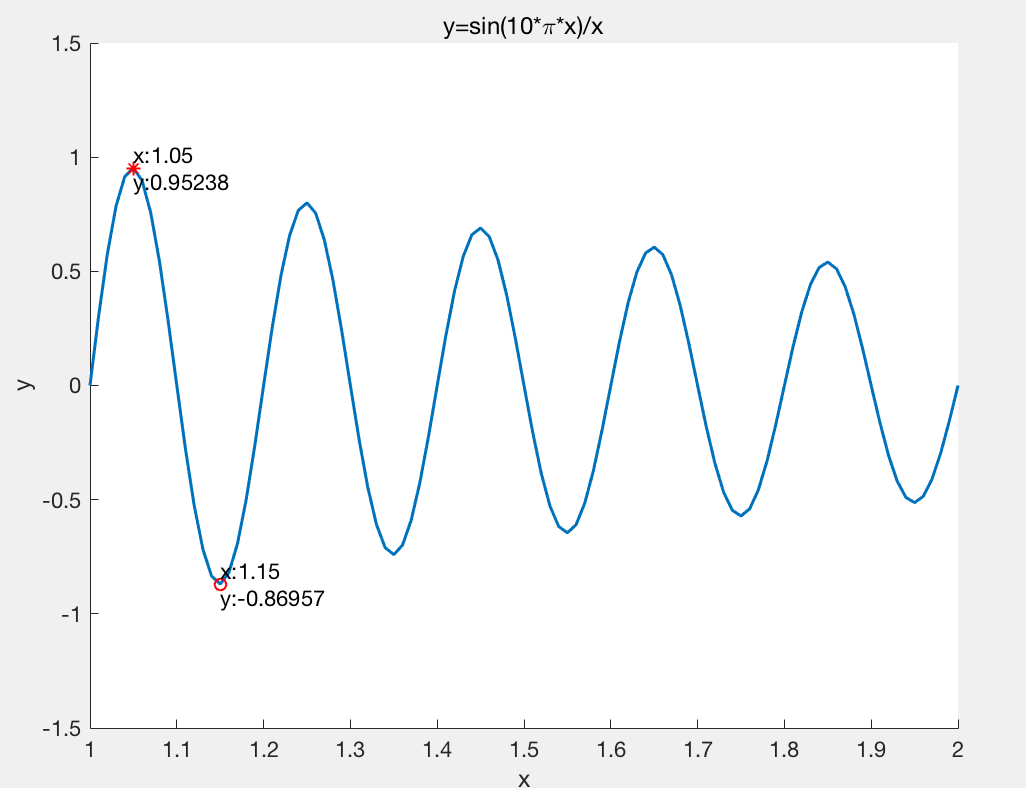
求y=sin(10*pi*x)./x;在[1,2]的最值
下图是用画图法求出最值的
x=1:0.01:2;
y=sin(10*pi*x)./x;
figure
hold on
plot(x,y,'linewidth',1.5);
ylim([-1.5,1.5]);
xlabel('x');
ylabel('y');
title('y=sin(10*pi*x)/x');
[maxVal,maxIndex]=max(y);
plot(x(maxIndex),maxVal,'r*');
text(x(maxIndex),maxVal,{['x:' num2str(x(maxIndex))],['y:' num2str(maxVal)]});
[minVal,minIndex]=min(y);
plot(x(minIndex),minVal,'ro');
text(x(minIndex),minVal,{['x:' num2str(x(minIndex))],['y:' num2str(minVal)]});
hold off;
用模拟退火工具箱来找最值
求最小值
function fitness=fitnessfun(x)
fitness=sin(10*pi*x)./x;
end
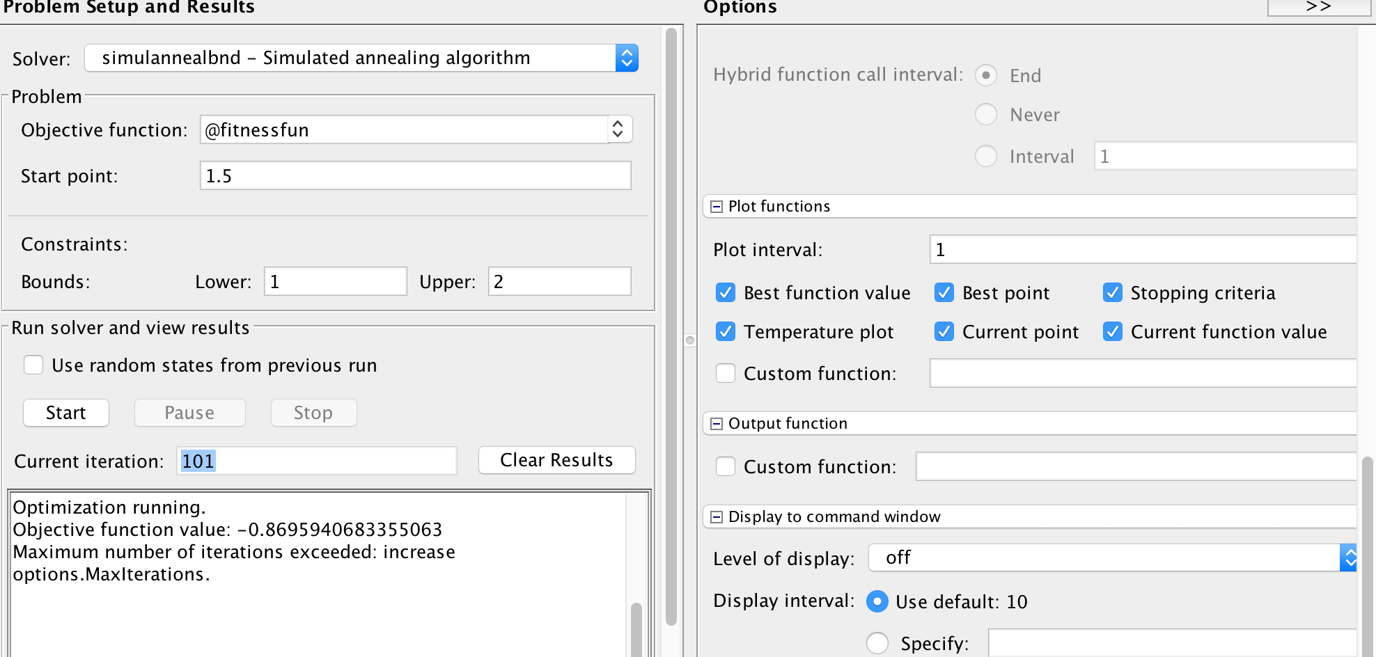
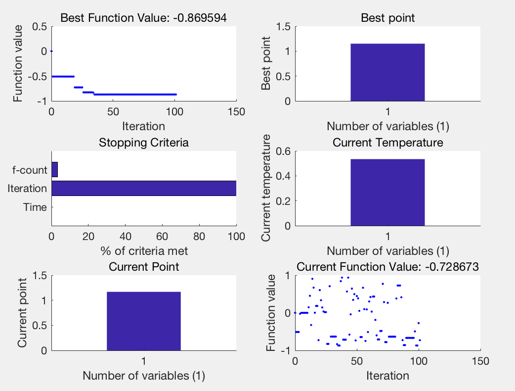
求最大值
function fitness=fitnessfun(x)
fitness=-sin(10*pi*x)./x;
end
Optimization running.
Objective function value: -0.9527670052175917
Maximum number of iterations exceeded: increase options.MaxIterations.
用工具箱求得的最大值为0.9527670052175917
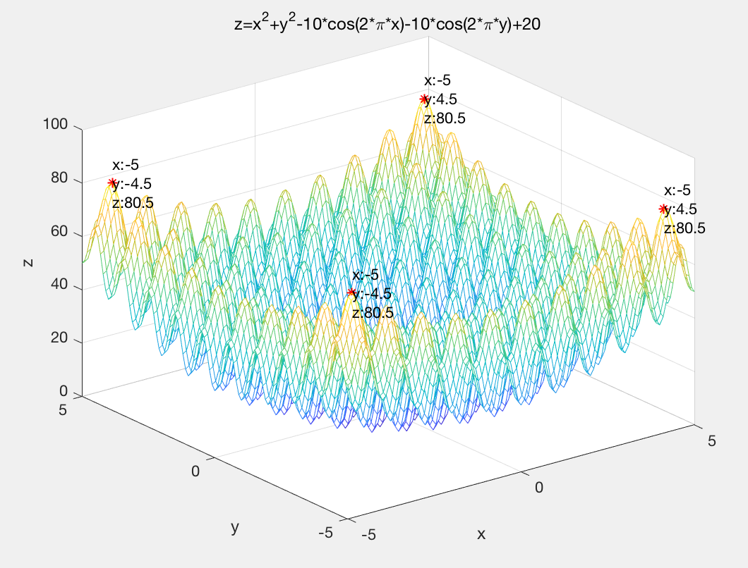
2.二元函数优化
[x,y]=meshgrid(-5:0.1:5,-5:0.1:5);
z=x.^2+y.^2-10*cos(2*pi*x)-10*cos(2*pi*y)+20;
figure
mesh(x,y,z);
hold on
xlabel('x');
ylabel('y');
zlabel('z');
title('z=x^2+y^2-10*cos(2*pi*x)-10*cos(2*pi*y)+20');
maxVal=max(z(:));
[maxIndexX,maxIndexY]=find(z==maxVal);%返回z==maxVal时,x和y的索引
for i=1:length(maxIndexX)
    plot3(x(maxIndexX(i),maxIndexY(i)),y(maxIndexX(i),maxIndexY(i)),maxVal,'r*');
    text(x(maxIndexX(i),maxIndexY(i)),y(maxIndexX(i),maxIndexY(i)),maxVal,{['x:' num2str(x(maxIndexX(i)))] ['y:' num2str(y(maxIndexY(i)))] ['z:' num2str(maxVal)] });
end
hold off;
function fitness=fitnessfun(x)
fitness=-(x(1).^2+x(2).^2-10*cos(2*pi*x(1))-10*cos(2*pi*x(2))+20);
end
Optimization running.
Objective function value: -80.50038894455415
Maximum number of iterations exceeded: increase options.MaxIterations.
找到的最大值:80.50038894455415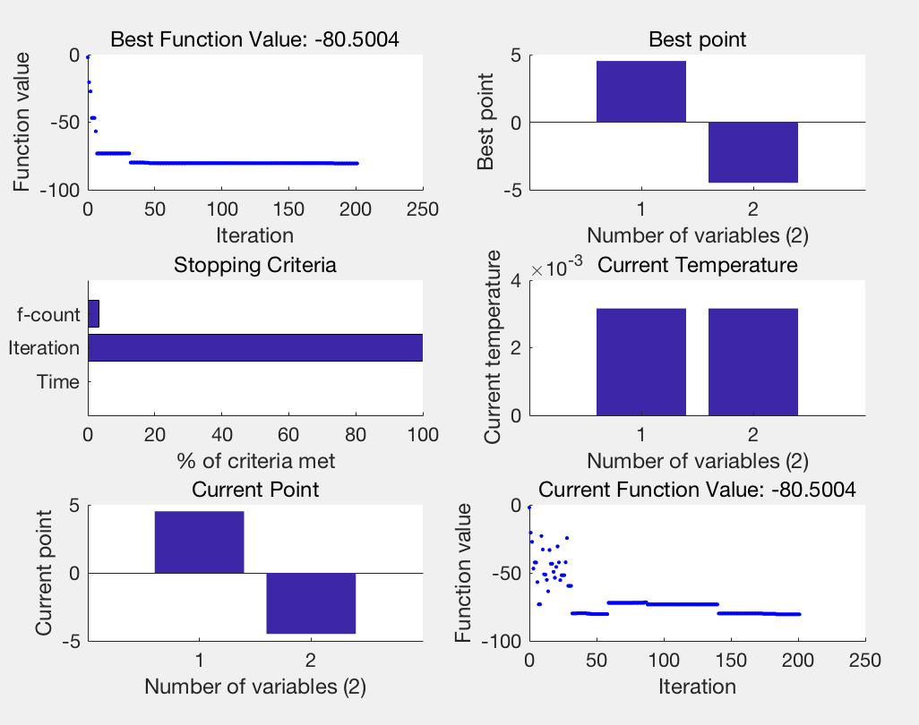
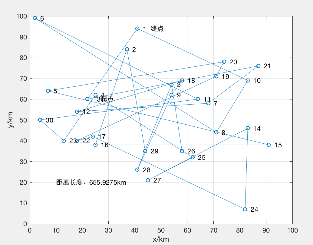
3.解TSP问题
(用的数据和前几天用遗传算法写TSP问题的数据一致,但是结果比遗传算法算出来效果差很多,不知道是不是我写错了,怀疑人生_(:з」∠)_中。。。
x=[41 94;37 84;54 67;25 62;7 64;2 99;68 58;71 44;54 62;83 69;64 60;18 54;22 60;
83 46;91 38;25 38;24 42;58 69;71 71;74 78;87 76;18 40;13 40;82 7;62 32;58 35;45 21;41 26;44 35;4 50];
d=distance(x);%计算距离矩阵
n=size(d,1);%城市的个数
T0=1e50;%初始温度
Tend=1e-30;%终止温度
L=2;%各温度下的迭代次数
q=0.95;
%计算迭代的次数 T0 * (0.95)^x = Tf
time=ceil(double(solve([num2str(T0) '*(0.9)^x=' num2str(Tend)])));%计算迭代的参数
count=0;
obj=zeros(time,1);
path=zeros(time,n);
%随机产生一条初始路线
journey=randperm(n);
rlength=pathlength(d,journey);
drawpath(journey,x,rlength);
disp('初始种群中的一个随机值:');
outputpath(journey);
disp(['初始路径总距离:',num2str(rlength)]);
index=0;
%迭代优化
while T0>Tend
count=count+1;
%产生新解
newjourney=NewAnswer(journey);
[journey,r]=Metropolis(journey,newjourney,d,T0);
%记录每次迭代的最优路线
if count==1||r<obj(count-1)
obj(count)=r;
index=count;
else
obj(count)=obj(count-1);
end
path(count,:)=journey;
T0=T0*q;
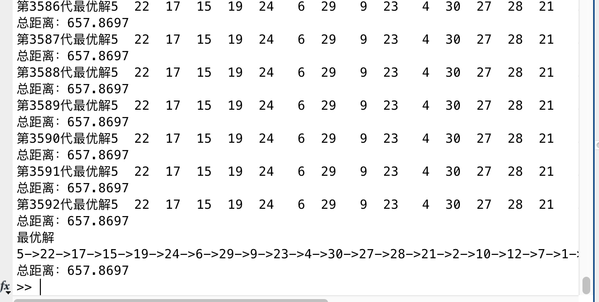
disp(['第' num2str(count) '代最优解' num2str(path(count,:))] );
disp(['总距离:',num2str(obj(count))]);
end
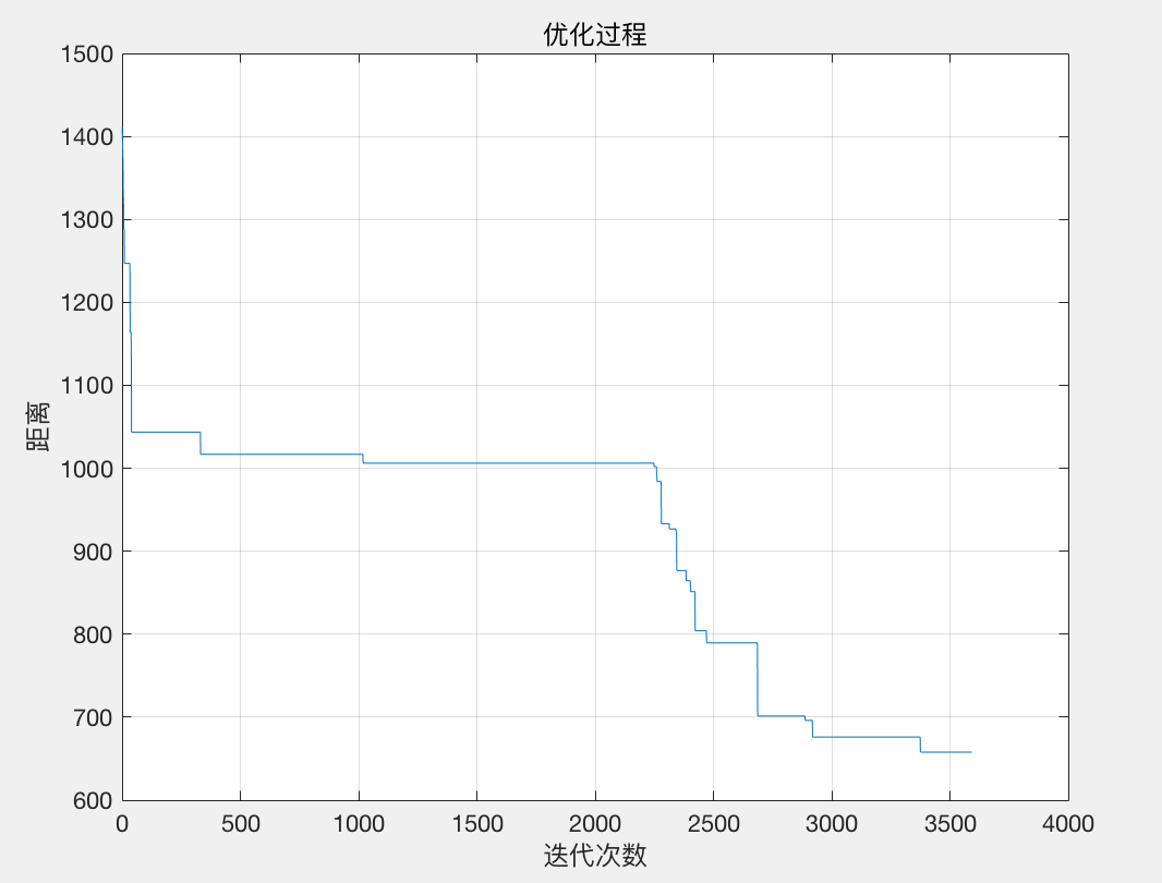
figure
plot(1:count,obj);
xlabel('迭代次数');
ylabel('距离');
title('优化过程');
grid on;
s=path(index,:);
a=pathlength(d,s);
drawpath(path(index,:),x,a);
disp('最优解');
p=outputpath(s);
disp(['总距离:',num2str(a)]);
function d=distance(citys)
%输入 各城市的位置坐标
%输出 两两城市之间的距离
n=size(citys,1);
d=zeros(n,n);
for i=1:n
    for j=1:n
        d(i,j)=((citys(i,1)-citys(j,1))^2+(citys(i,2)-citys(j,2))^2)^0.5;
        d(j,i)=d(i,j);
    end
end
function [s,r]=Metropolis(s1,s2,d,t)
%s1 当前解
%s2 新解
%d 距离矩阵
%t 温度
%s 下一个当前解
%r 下一个当前解的路线距离
r1=pathlength(d,s1);%计算s1路线长度
n=size(d(2));%城市的个数
r2=pathlength(d,s2);%计算s2路线长度
dc=r2-r1;%计算能力之差

%比前一个解更优接受新解,没有前一个解以一定概率接受新解
if dc<0
    s=s2;
    r=r2;
elseif exp(-dc/t)>0 % 以exp(-dC/T)概率接受新路线
        a=exp(-dc/t)*100;
        test(1:100)=0;
        test(1:a)=1;
        r=round(99*rand+1);
        pcc=test(r);
        if pcc==1
        s=s2;
        r=r2;
        else
            s=s1;
            r=r1;
        end
    else
        s=s1;
        r=r1;
end
end
function s2=NewAnswer(s1)
%随机产生新的解
%s1 当前解
%s2 新解
n=length(s1);
s2=s1;
a=round(rand(1,2)*(n-1)+1);
s2(a(2))=s1(a(1));
w=s1(a(2));
s2(a(1))=w;
function p=outputpath(route)
%给R末端添加起点R(1)
route=[route,route(1)];
n=length(route);
p=num2str(route(1));
for i=2:n
p=[p,'->',num2str(route(i))];
end
disp(p);
function dis=pathlength(d,route)
%计算起点与终点之间的距离
%d 城市间距离
%route 路线
dis=0;
n=length(d);
for i=1:n-1
    j=route(i);
    k=route(i+1);
   dis=dis+d(route(j),route(k));

end
j=route(n);
dis=dis+d(route(1),route(j));
function drawpath(route,citys,s)
%传入参数 路线 城市坐标
figure
plot([citys(route, 1); citys(route(1), 1)], [citys(route, 2); citys(route(1), 2)], 'o-');
grid on

%给每个地点标上序号
for i = 1: size(citys, 1)
    text(citys(i, 1), citys(i, 2), ['   ' num2str(i)]);
end

text(citys(route(1), 1), citys(route(1), 2), '       起点');
text(citys(route(end), 1), citys(route(end), 2), '       终点');
text(10,20,['距离长度:' num2str(s) 'km']);
xlabel('x/km');
ylabel('y/km');