关于感受野 (Receptive field) 你该知道的事

Receptive field 可中译为“感受野”，是卷积神经网络中非常重要的概念之一。

我个人最早看到这个词的描述是在 2012 年 Krizhevsky 的 paper 中就有提到过，当时是各种不明白的，事实上各种网络教学课程也都并没有仔细的讲清楚“感受野”是怎么一回事，有什么用等等。直到我某天看了 UiO 的博士生 Dang Ha The Hien写了一篇非常流传甚广的博文：A guide to receptive field arithmetic for Convolutional Neural Networks，才大彻大悟，世界变得好了，人生都变得有意义了，正如博主自己谈到的写作动机：

This post fills in the gap by introducing a new way to visualize feature maps in a CNN that exposes the receptive field information, accompanied by a complete receptive field calculation that can be used for any CNN architecture.

此文算是上述博文的一个精要版笔记，再加上个人的理解与计算过程。

FYI：读者已经熟悉 CNN 的基本概念，特别是卷积和池化操作。一个非常好的细致概述相关计算细节的 paper 是：A guide to convolution arithmetic for deep learning。

感受野可视化

我们知晓某一层的卷积核大小对应于在上一层输出的“图像”上的“视野”大小。比如，某层有 3x3 的卷积核，那就是一个 3x3 大小的滑动窗口在该层的输入“图像”上去扫描，我们就可以谈相对于上一层，说该层下特征图（feature map）当中任一特征点（feature）的“感受野”大小只有 3x3.（打引号说明术语引用不够严谨）。

先看个感受野的较严格定义：

The receptive field is defined as the region in the input space that a particular CNN’s feature is looking at (i.e. be affected by).

一个特征点的感受野可以用其所在的中心点位置（center location）和大小（size）来描述。然而，某卷积特征点所对应的感受野上并不是所有像素都是同等重要的，就好比人的眼睛所在的有限视野范围内，总有要 focus 的焦点。对于感受野来说，距离中心点越近的像素肯定对未来输出特征图的贡献就越大。换句话说，一个特征点在输入图像（Input）上所关注的特定区域（也就是其对应的感受野）会在该区域的中心处聚焦，并以指数变化向周边扩展（need more explanation）。

废话不多说，我们直接先算起来。

首先假定我们所考虑的 CNN 架构是对称的，并且输入图像也是方形的。这样的话，我们就忽略掉不同长宽所造成的维度不同。

Way1 对应为通常的一种理解感受野的方式。在下方左侧的上图中，是在 5x5 的图像(蓝色)上做一个 3x3 卷积核的卷积计算操作，步长为2，padding 为1，所以输出为 3x3 的特征图(绿色)。那么该特征图上的每个特征(1x1)对应的感受野，就是 3x3。在下方左侧的下图中，是在上述基础上再加了一个完全一样的卷积层。对于经过第二层卷积后其上的一个特征(如红色圈)在上一层特征图上“感受”到 3x3 大小，该 3x3 大小的每个特征再映射回到图像上，就会发现由 7x7 个像素点与之关联，有所贡献。于是，就可以说第二层卷积后的特征其感受野大小是 7x7（需要自己画个图，好好数一数）。Way2 （下方右侧的图像）是另一种理解的方式，主要的区别仅仅是将两层特征图上的特征不进行“合成”，而是保留其在前一层因“步长”而产生的影响。

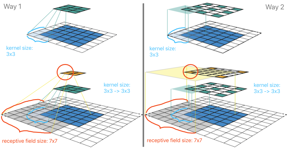
Way2 的理解方式其实更具有一般性，我们可以无需考虑输入图像的大小对感受野进行计算。如下图：

虽然，图上绘制了输入 9x9 的图像（蓝色），但是它的大小情况是无关紧要的，因为我们现在只关注某“无限”大小图像某一像素点为中心的一块区域进行卷积操作。首先，经过一个 3x3 的卷积层（padding=1，stride=2）后，可以得到特征输出（深绿色）部分。其中深绿色的特征分别表示卷积核扫过输入图像时，卷积核中心点所在的相对位置。此时，每个深绿色特征的感受野是 3x3 （浅绿）。这很好理解，每一个绿色特征值的贡献来源是其周围一个 3x3 面积。再叠加一个 3x3 的卷积层（padding=1，stride=2）后，输出得到 3x3 的特征输出（橙色）。此时的中心点的感受野所对应的是黄色区域 7x7，代表的是输入图像在中心点橙色特征所做的贡献。

这就是为何在《VERY DEEP CONVOLUTIONAL NETWORKS FOR LARGE-SCALE IMAGE RECOGNITION》文章中提到：

It is easy to see that a stack of two 3 × 3 conv. layers (without spatial pooling in between) has an effective receptive field of 5 × 5; three such layers have a 7 × 7 effective receptive field.

也就是说两层 3x3 的卷积层直接堆叠后（无池化）可以算的有感受野是 5x5，三层堆叠后的感受野就是 7x7。

感受野计算

直观的感受了感受野之后，究竟该如何定量计算嗯？只要依据 Way2 图像的理解，我们对每一层的特征“顺藤摸瓜”即可。

我们已经发觉到，某一层特征上的感受野大小依赖的要素有：每一层的卷积核大小 k，padding 大小 p，stride s。在推导某层的感受野时，还需要考虑到该层之前各层上特征的的感受野大小 r，以及各层相邻特征之间的距离 j（jump）。

所以对于某一卷积层（卷积核大小 k，padding 大小 p，stride s）上某特征的感受野大小公式为：

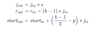
第一行计算的是，相邻特征之间的距离（jump）。各层里的特征之间的距离显然是严重依赖于 stride 的，并且逐层累积。值得注意的是，输入图像的作为起始像素特征，它的特征距离（jump）为1。
第二行计算的就是某层的特征的感受大小。它依赖于上一层的特征的感受野大小
第三行公式计算的是特征感受野的几何半径。对于处于特征图边缘处的特征来说，这类特征的感受野并不会完整的对应到原输入图像上的区域，都会小一些。初始特征的感受野几何半径为 0.5。

下面，我们继续拿可视化时用的例子，看看具体是怎么计算和对应的：

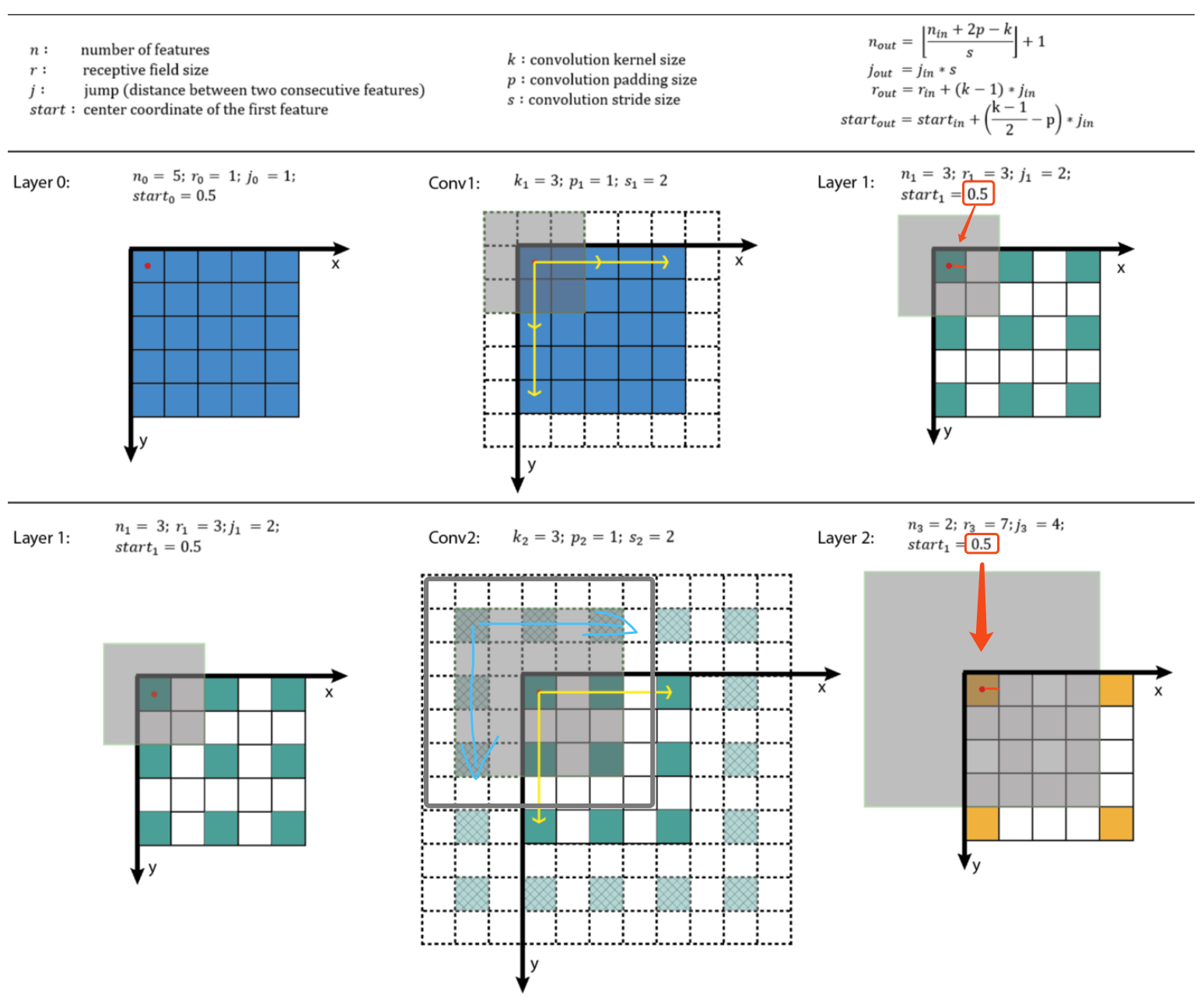
上图中除了公式和说明部分外，有两行分别代表的是第一层卷积和第二层卷积。在每行中，应从左往右观察卷积核计算和操作。

第一层比较简单，最后输出 3x3 绿色的特征图，每个特征有阴影框大小来表示每个特征对应的感受野大小 3x3。其中表示的 0.5 几何半径，我已经用红色标识出来，对应于阴影面积覆盖到的绿色面积的几何半径。

第二层，由于有一个单位的 padding，所以 3x3 卷积核是按照蓝色箭头标记作为的起始方向开始，在所有的绿色位置上挪动的。最后算得特征的感受野大小为 7x7，亦对应于阴影框和阴影区域部分。其中

Python Script

这个代码其实很好写，我就直接挪用 Dang Ha The Hien 的 python 脚本了：

# [filter size, stride, padding]
#Assume the two dimensions are the same
#Each kernel requires the following parameters:
# - k_i: kernel size
# - s_i: stride
# - p_i: padding (if padding is uneven, right padding will higher than left padding; "SAME" option in tensorflow)
# 
#Each layer i requires the following parameters to be fully represented: 
# - n_i: number of feature (data layer has n_1 = imagesize )
# - j_i: distance (projected to image pixel distance) between center of two adjacent features
# - r_i: receptive field of a feature in layer i
# - start_i: position of the first feature's receptive field in layer i (idx start from 0, negative means the center fall into padding)

import math
convnet =   [[11,4,0],[3,2,0],[5,1,2],[3,2,0],[3,1,1],[3,1,1],[3,1,1],[3,2,0],[6,1,0], [1, 1, 0]]
layer_names = ['conv1','pool1','conv2','pool2','conv3','conv4','conv5','pool5','fc6-conv', 'fc7-conv']
imsize = 227

def outFromIn(conv, layerIn):
  n_in = layerIn[0]
  j_in = layerIn[1]
  r_in = layerIn[2]
  start_in = layerIn[3]
  k = conv[0]
  s = conv[1]
  p = conv[2]
  
  n_out = math.floor((n_in - k + 2*p)/s) + 1
  actualP = (n_out-1)*s - n_in + k 
  pR = math.ceil(actualP/2)
  pL = math.floor(actualP/2)
  
  j_out = j_in * s
  r_out = r_in + (k - 1)*j_in
  start_out = start_in + ((k-1)/2 - pL)*j_in
  return n_out, j_out, r_out, start_out
  
def printLayer(layer, layer_name):
  print(layer_name + ":")
  print("	 n features: %s 
 	 jump: %s 
 	 receptive size: %s 	 start: %s " % (layer[0], layer[1], layer[2], layer[3]))
 
layerInfos = []
if __name__ == '__main__':
#first layer is the data layer (image) with n_0 = image size; j_0 = 1; r_0 = 1; and start_0 = 0.5
  print ("-------Net summary------")
  currentLayer = [imsize, 1, 1, 0.5]
  printLayer(currentLayer, "input image")
  for i in range(len(convnet)):
    currentLayer = outFromIn(convnet[i], currentLayer)
    layerInfos.append(currentLayer)
    printLayer(currentLayer, layer_names[i])
  print ("------------------------")
  layer_name = raw_input ("Layer name where the feature in: ")
  layer_idx = layer_names.index(layer_name)
  idx_x = int(raw_input ("index of the feature in x dimension (from 0)"))
  idx_y = int(raw_input ("index of the feature in y dimension (from 0)"))
  
  n = layerInfos[layer_idx][0]
  j = layerInfos[layer_idx][1]
  r = layerInfos[layer_idx][2]
  start = layerInfos[layer_idx][3]
  assert(idx_x < n)
  assert(idx_y < n)
  
  print ("receptive field: (%s, %s)" % (r, r))
  print ("center: (%s, %s)" % (start+idx_x*j, start+idx_y*j))

在 AlexNet 网络上的效果如下：