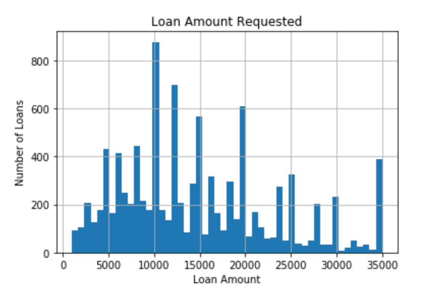
# data is a DataFrame type

data.sample(nums)     # 随机取nums个值

data.col.unique()        # 返回col取的所有值

#对于变量(不论连续或者离散或者类型变量), 得到其col的取值直方图
fig = data.loan_amnt.hist(bins=50)   # loan_amnt is a col in data
fig.set_title('loan Amount hist')
fig.set_xlabel('loan Amount')
fig.set_ylabel('Number of Loans')
data.open_acc.dropna().unique() # col dropna() 删去所有含有缺失值的

np.where(binary_array, 1, 0) # binary_array中为True的用1代替,其他的用0代替

data['defaulted'] = np.where(data.loan_status.isin(['Default']), 1, 0)

data.loan_status.isin(['Default']) # 判断loan_status是否是‘Default’,返回列表
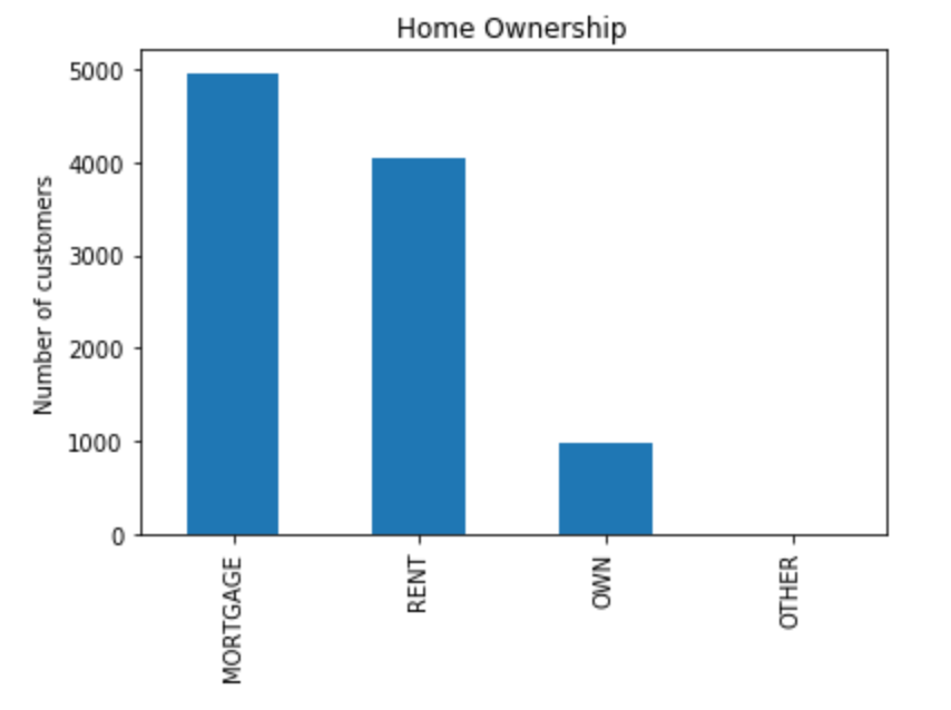
data['col'].value_counts()

# for each category of home ownership

fig = data['home_ownership'].value_counts().plot.bar()
fig.set_title('Home Ownership')
fig.set_ylabel('Number of customers')
data.groupby([col])['y'].sum()
缺失值
data.isnull().sum() # 计算每个col中为null的数目

data.isnull().mean() #计算每个col中null数据所占比例

data['cabin_null'] = np.where(data.Cabin.isnull(), 1, 0)

data.groupby(['Survived'])['cabin_null'].mean()

data['emp_length_redefined'] = data.emp_length.map(length_dict)

data.emp_length_redefined.unique()

data[data.emp_title.isnull()].groupby(['emp_length_redefined'])['emp_length'].count().sort_values() / value
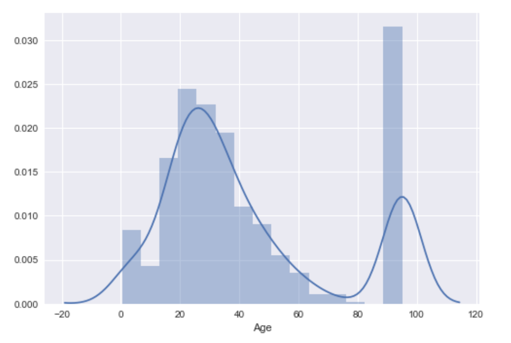
Outliers
import seaborn as sns
sns.distplot(data.Age)
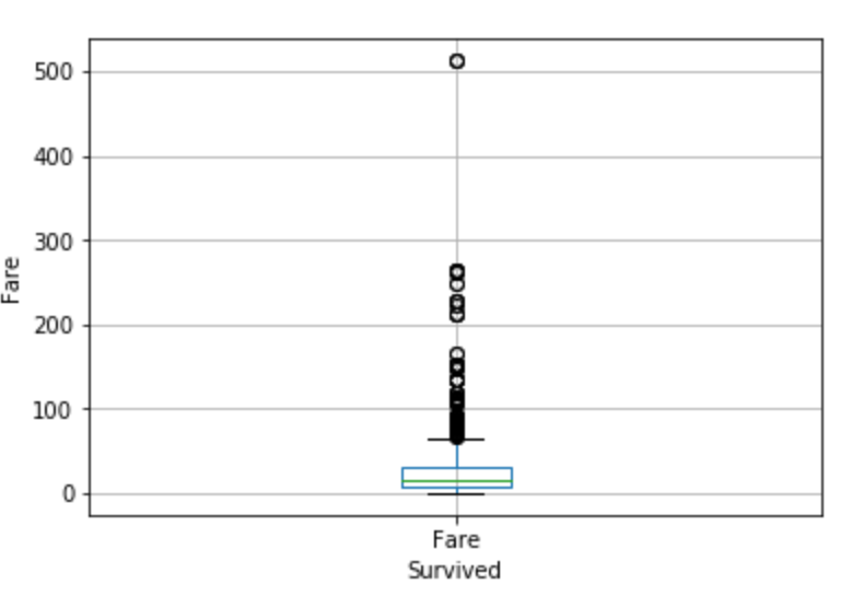
# another way of visualising outliers is using boxplots and whiskers,
# which provides the quantiles (box) and inter-quantile range (whiskers),
# with the outliers sitting outside the error bars (whiskers).

# All the dots in the plot below are outliers according to the quantiles + 1.5 IQR rule

fig = data.boxplot(column='Fare')
fig.set_title('')
fig.set_xlabel('Survived')
fig.set_ylabel('Fare')
# let's look at the values of the quantiles so we can
# calculate the upper and lower boundaries for the outliers

# 25%, 50% and 75% in the output below indicate the
# 25th quantile, median and 75th quantile respectively

data.Fare.describe()
# Let's calculate the upper and lower boundaries
# to identify outliers according
# to interquantile proximity rule

IQR = data.Fare.quantile(0.75) - data.Fare.quantile(0.25)

Lower_fence = data.Fare.quantile(0.25) - (IQR * 1.5)
Upper_fence = data.Fare.quantile(0.75) + (IQR * 1.5)

Upper_fence, Lower_fence, IQR
multiple_tickets = pd.concat(
    [
        high_fare_df.groupby('Ticket')['Fare'].count(),
        high_fare_df.groupby('Ticket')['Fare'].mean()
    ],
    axis=1)

multiple_tickets.columns = ['Ticket', 'Fare']
multiple_tickets.head(10)
Rare Values
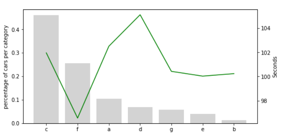
 Let's make a combined plot of the label frequency and
# the time to pass testing.
# This will help us  visualise the relationship between the
# target and the labels of X3

fig, ax = plt.subplots(figsize=(8, 4))
plt.xticks(temp_df.index, temp_df['X3'], rotation=0)

ax2 = ax.twinx()
ax.bar(temp_df.index, temp_df["X3_perc_cars"], color='lightgrey')
ax2.plot(temp_df.index, temp_df["y"], color='green', label='Seconds')
ax.set_ylabel('percentage of cars per category')
ax2.set_ylabel('Seconds')
# let's automate the above process for all the categorical variables

for col in cols_to_use:
    # calculate the frequency of the different labels in the variable
    temp_df = pd.Series(data[col].value_counts() / total_cars).reset_index()

    # rename the columns
    temp_df.columns = [col, col + '_perc_cars']

    # merge onto the mean time to pass the test
    temp_df = temp_df.merge(
        data.groupby([col])['y'].mean().reset_index(), on=col, how='left')

    # plot the figure as shown above
    fig, ax = plt.subplots(figsize=(8, 4))
    plt.xticks(temp_df.index, temp_df[col], rotation=0)
    ax2 = ax.twinx()

    ax.bar(
        temp_df.index,
        temp_df[col + '_perc_cars'],
        color='lightgrey',
        label=col)

    ax2.plot(
        temp_df.index,
        temp_df["y"],
        color='green',
    )

    ax.set_ylabel('percentage of cars per category')
    ax2.set_ylabel('Seconds')
    ax.legend()
    plt.show()
# let's automate the replacement of infrequent categories
# by the label 'rare' in the remaining categorical variables

# I start from 1 because I already replaced the first variable in
# the list
for col in cols_to_use[1:]:

    # calculate the % of cars in each category
    temp_df = pd.Series(data[col].value_counts() / total_cars)

    # create a dictionary to replace the rare labels with the
    # string 'rare'
    grouping_dict = {
        k: ('rare' if k not in temp_df[temp_df >= 0.1].index else k)
        for k in temp_df.index
    }

    # replace the rare labels
    data[col + '_grouped'] = data[col].map(grouping_dict)

data.head()
# In order to use this variables to build machine learning using sklearn
# first we need to replace the labels by numbers.

# The correct way to do this, is to first separate into training and test
# sets. And then create a replacing dictionary using the train set
# and replace the strings both in train and test using the dictionary
# created.

# This will lead to the introduction of missing values / NaN in the
# test set, for those labels that are not present in the train set
# we saw this effect in the previous lecture

# in the section dedicated to rare values later in the course, I will
# show you how to avoid this problem

# now, in order to speed up the demonstration, I will replace the
# labels by strings in the entire dataset, and then divide into
# train and test.
# but remember: THIS IS NOT GOOD PRACTICE!

# original variables
for col in cols_to_use:
    # create the dic and replace the strings in one line
    data.loc[:, col] = data.loc[:, col].map(
        {k: i
         for i, k in enumerate(data[col].unique(), 0)})

# variables with grouped categories
for col in ['X1_grouped', 'X6_grouped', 'X3_grouped', 'X2_grouped']:
    # create the dic and replace the strings in one line
    data.loc[:, col] = data.loc[:, col].map(
        {k: i
         for i, k in enumerate(data[col].unique(), 0)})
# let's capture the first letter
data['Cabin_reduced'] = data['Cabin'].astype(str).str[0]
# Now I will replace the letters in the reduced cabin variable

# create replace dictionary
cabin_dict = {k: i for i, k in enumerate(X_train['Cabin_reduced'].unique(), 0)}

# replace labels by numbers with dictionary
X_train.loc[:, 'Cabin_reduced'] = X_train.loc[:, 'Cabin_reduced'].map(cabin_dict)
X_test.loc[:, 'Cabin_reduced'] = X_test.loc[:, 'Cabin_reduced'].map(cabin_dict)