警告:本文为小白入门学习笔记
数据连接:
数据集是(x(i),y(i))
x = load('ex2x.dat');
y = load('ex2y.dat');

plot(x, y, 'o');

假设函数(hypothesis function):

接下来用矩阵的形式表示x:
m = length(y); % store the number of training examples
x = [ones(m, 1), x]; % Add a column of ones to x

MATLAB实现:
function [jVal,gradient] = linerCost(theta)
x = load('ex2x.dat');
y = load('ex2y.dat');
m = length(y); % store the number of training examples
%x = [ones(m, 1), x]; % Add a column of ones to x
w = 0;
for i = 1:m
w = w + (theta(1) + theta(2) .* x(i) - y(i)).^2;
end
jVal = 1./2 .* m .* w;
gradient = zeros(2,1);
w = 0;
for i = 1:m
w = w + (theta(1) + theta(2) .* x(i) - y(i));
end
gradient(1) = w;
w = 0;
for i = 1:m
w = w + (theta(1) + theta(2) .* x(i) - y(i)).*x(i);
end
gradient(2) = w;
end
命令控制台:
>> options = optimset('GradObj','on','MaxIter',1000);
>> initialTheta = zeros(2,1);
>> [optTheta,functionVal,exitFlag] = fminunc(@costFunction,initialTheta ,options)
返回结果:
optTheta =
0.7502
0.0639
functionVal =
2.4677
exitFlag =
1
由于本案例只有一个feature,所以还可以在二维平面上查看结果,如果是高维度就无法看结果。

本实验中,theta的选择,和learning rate的选取都是由MATLAB自动实现的;
如果要自己手写
for i = 1:iter
theta = theta - X'*(X*theta-y)/m*alpha;
end
需要自己选取alpha,还有确定迭代的次数iter
如果使用矩阵直接计算会更加快而且准确(对于本题而言):
![]()
入门菜鸟,错误地方欢迎指教!
补充
局部加权线性回归
如果是以下数据集

左图可以看出,这是一种欠拟合的现象,怎么才能使拟合的更好呢?
使用高斯核 的 局部加权线性回归
高斯函数是
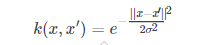
随着x与x′的距离的距离的增大,其高斯核函数值在单调递减。根据这个特点,可以对预测点在附近的每一点赋值,离预测点越近的点权重越大
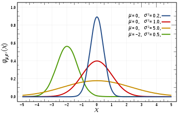
用下面图说明
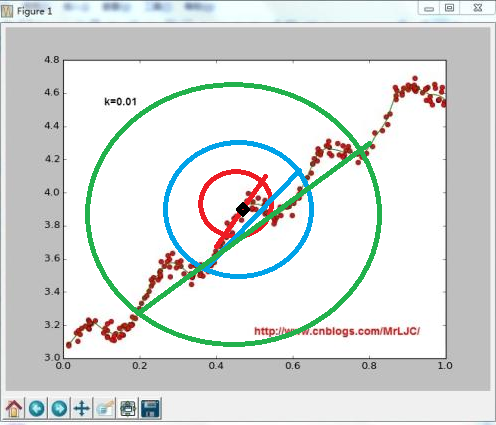
图中设黑色点是预测点,红色区域σ的值最小,随着σ的增大影响范围也在增大,而它的拟合曲线也在改变
所以可以通过改变σ的值来调整拟合的情况
整体来说,σ=1时把所有的点都包含,局部加权没有作用
当σ过小时会出现欠拟合现象
普通正规矩阵回归曲线
局部加权线性回归
岭回归
代码+注释
#coding=utf-8
from numpy import *
import matplotlib.pyplot as plt

#加载数据
def loadDataSet(fileName):
    numFeat = len(open(fileName).readline().split('	')) - 1
    dataMat = []; labelMat = []
    fr = open(fileName)
    for line in fr.readlines():
        lineArr =[]
        curLine = line.strip().split('	')
        for i in range(numFeat):
            lineArr.append(float(curLine[i]))
        dataMat.append(lineArr)
        labelMat.append(float(curLine[-1]))
    return dataMat,labelMat

#使用正规矩阵来计算回归系数w(w[0]是系数b,w[1]是斜率k)
def standRegres(xArr,yArr):
    xMat = mat(xArr); yMat = mat(yArr).T
    xTx = xMat.T*xMat
    #不可逆判断
    if linalg.det(xTx) == 0.0:
        print ("This matrix is singular, cannot do inverse")
        return
    ws = xTx.I * (xMat.T*yMat)
    return ws

#使用局部加权的线性回归
def lwlr(testPoint,xArr,yArr,k=1.0):
    xMat = mat(xArr); yMat = mat(yArr).T
    m = shape(xMat)[0]
    weights = mat(eye((m)))
    #为每一个样本点增加权重
    for j in range(m):
        diffMat = testPoint - xMat[j,:]
        #使用高斯核函数来加权
        weights[j,j] = exp(diffMat*diffMat.T/(-2.0*k**2))
    xTx = xMat.T * (weights * xMat)
    if linalg.det(xTx) == 0.0:
        print ("This matrix is singular, cannot do inverse")
        return
    ws = xTx.I * (xMat.T * (weights * yMat))
    return testPoint * ws

#循环测试每一个点testPoint
def lwlrTest(testArr,xArr,yArr,k=1.0):
    m = shape(testArr)[0]
    yHat = zeros(m)
    for i in range(m):
        yHat[i] = lwlr(testArr[i],xArr,yArr,k)
    return yHat

#岭回归
def rssError(yArr,yHatArr):
    return ((yArr-yHatArr)**2).sum()

def ridgeRegres(xMat,yMat,lam=0.2):
    xTx = xMat.T*xMat
    #增加一个m*m的单位矩阵乘lambda默认值是0.2
    denom = xTx + eye(shape(xMat)[1])*lam
    if linalg.det(denom) == 0.0:
        print ("This matrix is singular, cannot do inverse")
        return
    ws = denom.I * (xMat.T*yMat)
    return ws

#不断的调增lambd的取值(增加),测试结果
def ridgeTest(xArr,yArr):
    xMat = mat(xArr); yMat=mat(yArr).T
    yMean = mean(yMat,0)
    yMat = yMat - yMean     #to eliminate X0 take mean off of Y
    #regularize X's
    xMeans = mean(xMat,0)   #calc mean then subtract it off
    xVar = var(xMat,0)      #calc variance of Xi then divide by it
    xMat = (xMat - xMeans)/xVar
    numTestPts = 30
    wMat = zeros((numTestPts,shape(xMat)[1]))
    for i in range(numTestPts):
        ws = ridgeRegres(xMat,yMat,exp(i-10))
        wMat[i,:]=ws.T
    return wMat

#前向逐步向前线性回归
def regularize(xMat):#regularize by columns
    inMat = xMat.copy()
    inMeans = mean(inMat,0)   #calc mean then subtract it off
    inVar = var(inMat,0)      #calc variance of Xi then divide by it
    inMat = (inMat - inMeans)/inVar
    return inMat

def stageWise(xArr,yArr,eps=0.01,numIt=100):
    xMat = mat(xArr); yMat=mat(yArr).T
    yMean = mean(yMat,0)
    yMat = yMat - yMean     #can also regularize ys but will get smaller coef
    xMat = regularize(xMat)
    m,n=shape(xMat)
    #returnMat = zeros((numIt,n)) #testing code remove
    ws = zeros((n,1)); wsTest = ws.copy(); wsMax = ws.copy()
    for i in range(numIt):
        print ws.T
        lowestError = inf;
        for j in range(n):
            for sign in [-1,1]:
                wsTest = ws.copy()
                wsTest[j] += eps*sign
                yTest = xMat*wsTest
                rssE = rssError(yMat.A,yTest.A)
                if rssE < lowestError:
                    lowestError = rssE
                    wsMax = wsTest
        ws = wsMax.copy()
        returnMat[i,:]=ws.T
    return returnMat

def test1():
    xArr,yArr = loadDataSet('ex0.txt')
    ws = standRegres(xArr,yArr)
    xMat = mat(xArr)
    yMat = mat(yArr)
    yHat = xMat * ws
    #绘制数据集的散点图
    fig = plt.figure()
    ax = fig.add_subplot(111)
    ax.scatter(xMat[:,1].flatten().A[0],yMat.T[:,0].flatten().A[0])
    #绘制回归曲线
    xCopy = xMat.copy()
    xCopy.sort(0)
    yHat = xCopy * ws
    ax.plot(xCopy[:,1],yHat)
    plt.show()

#-------------分割线-----以上是普通线性回归曲线------------------------

def test2():
    xArr,yArr = loadDataSet('ex0.txt')
    print (yArr[0])
    #测试点xArr[0],在不同取值k下的ws
    lwlr(xArr[0],xArr,yArr,1.0)
    lwlr(xArr[0],xArr,yArr,0.001)
    #调整k的取值来获得不同的拟合曲线
    yHat = lwlrTest(xArr,xArr,yArr,0.003)
    xMat = mat(xArr)
    strInd = xMat[:,1].argsort(0)
    xSort = xMat[strInd][:,0,:]
    #绘制数据集的散点图
    fig = plt.figure()
    ax = fig.add_subplot(111)
    #绘制回归曲线
    ax.plot(xSort[:,1],yHat[strInd])
    ax.scatter(xMat[:,1].flatten().A[0],mat(yArr).T.flatten().A[0],s=2,c='red')
    plt.show()

#-------------分割线-----以上是局部加权线性回归曲线------------------------
def test3():
    abX,abY = loadDataSet('abalone.txt')
    ridgeWeights = ridgeTest(abX,abY)
    fig = plt.figure()
    ax = fig.add_subplot(111)
    #画出lambda的变化过程
    ax.plot(ridgeWeights)
    plt.show() #当lambda很小时,系数和普通回归一样,随着lambda增大,回归系数减小为零,可以在中间得到一个预测结果较好的lambda