import numpy as np
import os
os.chdir('../')
import matplotlib.pyplot as plt
%matplotlib inline
一.最大熵原理
最大熵的思想很朴素,即将已知事实以外的未知部分看做“等可能”的,而熵是描述“等可能”大小很合适的量化指标,熵的公式如下:
这里分布(p)的取值有(i)种情况,每种情况的概率为(p_i),下图绘制了二值随机变量的熵:
p=np.linspace(0.1,0.9,90)
def entropy(p):
    return -np.log(p)*p-np.log(1-p)*(1-p)
plt.plot(p,entropy(p))
[<matplotlib.lines.Line2D at 0x245a3d6d278>]
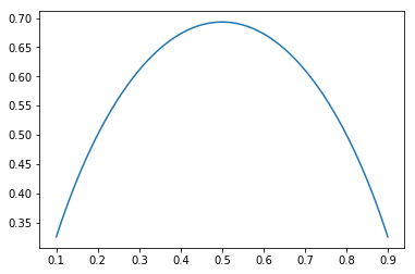
当两者概率均为0.5时,熵取得最大值,通过最大化熵,可以使得分布更“等可能”;另外,熵还有优秀的性质,它是一个凹函数,所以最大化熵其实是一个凸问题。
对于“已知事实”,可以用约束条件来描述,比如4个值的随机变量分布,其中已知(p_1+p_2=0.4),它的求解可以表述如下:
显然,最优解为:(p_1=0.2,p_2=0.2,p_3=0.3,p_4=0.3)
二.最大熵模型
最大熵模型是最大熵原理在分类问题上的应用,它假设分类模型是一个条件概率分布(P(Y|X)),即对于给定的输入(X),以概率(P(Y|X))输出(Y),这时最大熵模型的目标函数定义为条件熵:
这里,( ilde{P}(x))表示边缘分布(P(X))的经验分布,( ilde{P}(x)=frac{v(X=x)}{N}),(v(X=x))表示训练样本中输入(x)出现的次数,(N)表示训练样本的总数。
而最大熵模型的“已知事实”可以通过如下等式来约束:
为了方便,左边式子记着(E_P(f)),右边式子记着(E_{ ilde{P}}(f)),等式描述的是某函数(f(x,y))关于模型(P(Y|X))与经验分布( ilde{P}(X))的期望与函数(f(x,y))关于经验分布( ilde{P}(X,Y))的期望相同。(这里( ilde{P}(x,y)=frac{v(X=x,Y=y)}{N}))
所以重要的约束信息将由(f(x,y))来表示,它的定义如下:
故最大熵模型可以理解为,模型在某些事实发生的期望和训练集相同的条件下,使得条件熵最大化。所以,对于有(n)个约束条件的最大熵模型可以表示为:
按照优化问题的习惯,可以改写为如下:
由于目标函数为凸函数,约束条件为仿射,所以我们可以通过求解对偶问题,得到原始问题的最优解,首先引入拉格朗日乘子(w_0,w_1,...,w_n),定义拉格朗日函数(L(P,w)):
所以原问题等价于:
它的对偶问题:
首先,解里面的 (min_P L(P,w)),其实对于(forall w),(L(P,w))都是关于(P)的凸函数,因为(-H(P))是关于(P)的凸函数,而后面的(w_0(1-sum_yP(y|x)+sum_{i=1}^nw_i(E_{ ilde{P}}(f_i))-E_P(f_i)))是关于(P(y|x))的仿射函数,所以求(L(P,w))对(P)的偏导数,并令其等于0,即可解得最优的(P(y|x)),记为(P_w(y|x)),即:
在训练集中对任意样本(forall x,y),都有( ilde{P}(x)(logP(y|x)+1-w_0-sum_{i=1}^nw_if_i(x,y))=0),显然( ilde{P}(x)>0)((x)本来就是训练集中的一个样本,自然概率大于0),所以(logP(y|x)+1-w_0-sum_{i=1}^nw_if_i(x,y)=0),所以:
这就是最大熵模型的表达式(最后一步变换用到了(sum_y P(y|x)=1)),这里(w)即是模型的参数,聪明的童鞋其实已经发现,最大熵模型其实就是一个线性函数外面套了一个softmax函数,它大概就是如下图所示的这么回事:

接下来,将(L(P_w,w))带入外层的(max)函数,即可求解最优的参数(w^*):
推导一下模型的梯度更新公式:
这里,倒数第三步到倒数第二步用到了(sum_yP(y|x)=1),最后一步中(w=[w_1,w_2,...,w_n]^T,f(x,y)=[f_1(x,y),f_2(x,y),...,f_n(x,y)]^T),所以:
所以,自然(w)的更新公式:
这里,(eta)是学习率
三.对特征函数的进一步理解
上面推导出了最大熵模型的梯度更新公式,想必大家对(f(x,y))还是有点疑惑,“满足某一事实”这句话该如何理解?这其实与我们的学习目的相关,学习目的决定了我们的“事实”,比如有这样一个任务,判断“打”这个词是量词还是动词,我们收集了如下的语料:
| 句子/(x) | 目标/(y) |
|---|---|
| (x_1:)一打火柴 | (y_1:)量词 |
| (x_2:)三打啤酒 | (y_2:)量词 |
| (x_3:)打电话 | (y_3:) 动词 |
| (x_4:)打篮球 | (y_4:) 动词 |
通过观察,我们可以设计如下的两个特征函数来分别识别"量词"和"动词"任务:
当然,你也可以设计这样的特征函数来做识别“量词”的任务:
只是,这样的特征函数设计会使得模型学习能力变弱,比如遇到“三打火柴”,采用后面的特征函数设计就识别不出“打”是量词,而采用第一种特征函数设计就能很好的识别出来,所以要使模型具有更好的泛化能力,就需要设计更好的特征函数,而这往往依赖于人工经验,对于自然语言处理这类任务(比如上面的例子),我们可以较容易的归纳总结出一些有用的经验知识,但是对于其他情况,人工往往难以总结出一般性的规律,所以对于这些问题,我们需要设计更“一般”的特征函数。
一种简单的特征函数设计
我们可以简单考虑(x)的某个特征取某个值和(y)取某个类的组合做特征函数(对于连续型特征,可以采用分箱操作),所以我们可以设计这样两类特征函数:
(1)离散型:
(2)连续型:
四.代码实现
为了方便演示,首先构建训练数据和测试数据
# 测试
from sklearn import datasets
from sklearn import model_selection
from sklearn.metrics import f1_score

iris = datasets.load_iris()
data = iris['data']
target = iris['target']
X_train, X_test, y_train, y_test = model_selection.train_test_split(data, target, test_size=0.2,random_state=0)
为了方便对数据进行分箱操作,封装一个DataBinWrapper类,并对X_train和X_test进行转换(该类放到ml_models.wrapper_models中)
class DataBinWrapper(object):
    def __init__(self, max_bins=10):
        # 分段数
        self.max_bins = max_bins
        # 记录x各个特征的分段区间
        self.XrangeMap = None

    def fit(self, x):
        n_sample, n_feature = x.shape
        # 构建分段数据
        self.XrangeMap = [[] for _ in range(0, n_feature)]
        for index in range(0, n_feature):
            tmp = x[:, index]
            for percent in range(1, self.max_bins):
                percent_value = np.percentile(tmp, (1.0 * percent / self.max_bins) * 100.0 // 1)
                self.XrangeMap[index].append(percent_value)

    def transform(self, x):
        """
        抽取x_bin_index
        :param x:
        :return:
        """
        if x.ndim == 1:
            return np.asarray([np.digitize(x[i], self.XrangeMap[i]) for i in range(0, x.size)])
        else:
            return np.asarray([np.digitize(x[:, i], self.XrangeMap[i]) for i in range(0, x.shape[1])]).T
data_bin_wrapper=DataBinWrapper(max_bins=10)
data_bin_wrapper.fit(X_train)
X_train=data_bin_wrapper.transform(X_train)
X_test=data_bin_wrapper.transform(X_test)
X_train[:5,:]
array([[7, 6, 8, 7],
       [3, 5, 5, 6],
       [2, 8, 2, 2],
       [6, 5, 6, 7],
       [7, 2, 8, 8]], dtype=int64)
X_test[:5,:]
array([[5, 2, 7, 9],
       [5, 0, 4, 3],
       [3, 9, 1, 2],
       [9, 3, 9, 7],
       [1, 8, 2, 2]], dtype=int64)
由于特征函数可以有不同的形式,这里我们将特征函数解耦出来,构造一个SimpleFeatureFunction类(后续构造其他复杂的特征函数,需要定义和该类相同的函数名,该类放置到ml_models.linear_model中)
class SimpleFeatureFunction(object):
    def __init__(self):
        """
        记录特征函数
        {
            (x_index,x_value,y_index)
        }
        """
        self.feature_funcs = set()

    # 构建特征函数
    def build_feature_funcs(self, X, y):
        n_sample, _ = X.shape
        for index in range(0, n_sample):
            x = X[index, :].tolist()
            for feature_index in range(0, len(x)):
                self.feature_funcs.add(tuple([feature_index, x[feature_index], y[index]]))

    # 获取特征函数总数
    def get_feature_funcs_num(self):
        return len(self.feature_funcs)

    # 分别命中了那几个特征函数
    def match_feature_funcs_indices(self, x, y):
        match_indices = []
        index = 0
        for feature_index, feature_value, feature_y in self.feature_funcs:
            if feature_y == y and x[feature_index] == feature_value:
                match_indices.append(index)
            index += 1
        return match_indices
接下来对MaxEnt类进行实现,首先实现一个softmax函数的功能(ml_models.utils)
def softmax(x):
    if x.ndim == 1:
        return np.exp(x) / np.exp(x).sum()
    else:
        return np.exp(x) / np.exp(x).sum(axis=1, keepdims=True)
进行MaxEnt类的具体实现(ml_models.linear_model)
from ml_models import utils
class MaxEnt(object):
    def __init__(self, feature_func, epochs=5, eta=0.01):
        self.feature_func = feature_func
        self.epochs = epochs
        self.eta = eta

        self.class_num = None
        """
        记录联合概率分布:
        {
            (x_0,x_1,...,x_p,y_index):p
        }
        """
        self.Pxy = {}
        """
        记录边缘概率分布:
        {
            (x_0,x_1,...,x_p):p
        }
        """
        self.Px = {}

        """
        w[i]-->feature_func[i]
        """
        self.w = None

    def init_params(self, X, y):
        """
        初始化相应的数据
        :return:
        """
        n_sample, n_feature = X.shape
        self.class_num = np.max(y) + 1

        # 初始化联合概率分布、边缘概率分布、特征函数
        for index in range(0, n_sample):
            range_indices = X[index, :].tolist()

            if self.Px.get(tuple(range_indices)) is None:
                self.Px[tuple(range_indices)] = 1
            else:
                self.Px[tuple(range_indices)] += 1

            if self.Pxy.get(tuple(range_indices + [y[index]])) is None:
                self.Pxy[tuple(range_indices + [y[index]])] = 1
            else:
                self.Pxy[tuple(range_indices + [y[index]])] = 1

        for key, value in self.Pxy.items():
            self.Pxy[key] = 1.0 * self.Pxy[key] / n_sample
        for key, value in self.Px.items():
            self.Px[key] = 1.0 * self.Px[key] / n_sample

        # 初始化参数权重
        self.w = np.zeros(self.feature_func.get_feature_funcs_num())

    def _sum_exp_w_on_all_y(self, x):
        """
        sum_y exp(self._sum_w_on_feature_funcs(x))
        :param x:
        :return:
        """
        sum_w = 0
        for y in range(0, self.class_num):
            tmp_w = self._sum_exp_w_on_y(x, y)
            sum_w += np.exp(tmp_w)
        return sum_w

    def _sum_exp_w_on_y(self, x, y):
        tmp_w = 0
        match_feature_func_indices = self.feature_func.match_feature_funcs_indices(x, y)
        for match_feature_func_index in match_feature_func_indices:
            tmp_w += self.w[match_feature_func_index]
        return tmp_w

    def fit(self, X, y):
        self.eta = max(1.0 / np.sqrt(X.shape[0]), self.eta)
        self.init_params(X, y)
        x_y = np.c_[X, y]
        for epoch in range(self.epochs):
            count = 0
            np.random.shuffle(x_y)
            for index in range(x_y.shape[0]):
                count += 1
                x_point = x_y[index, :-1]
                y_point = x_y[index, -1:][0]
                # 获取联合概率分布
                p_xy = self.Pxy.get(tuple(x_point.tolist() + [y_point]))
                # 获取边缘概率分布
                p_x = self.Px.get(tuple(x_point))
                # 更新w
                dw = np.zeros(shape=self.w.shape)
                match_feature_func_indices = self.feature_func.match_feature_funcs_indices(x_point, y_point)
                if len(match_feature_func_indices) == 0:
                    continue
                if p_xy is not None:
                    for match_feature_func_index in match_feature_func_indices:
                        dw[match_feature_func_index] = p_xy
                if p_x is not None:
                    sum_w = self._sum_exp_w_on_all_y(x_point)
                    for match_feature_func_index in match_feature_func_indices:
                        dw[match_feature_func_index] -= p_x * np.exp(self._sum_exp_w_on_y(x_point, y_point)) / (
                            1e-7 + sum_w)
                # 更新
                self.w += self.eta * dw
                # 打印训练进度
                if count % (X.shape[0] // 4) == 0:
                    print("processing:	epoch:" + str(epoch + 1) + "/" + str(self.epochs) + ",percent:" + str(
                        count) + "/" + str(X.shape[0]))

    def predict_proba(self, x):
        """
        预测为y的概率分布
        :param x:
        :return:
        """
        y = []
        for x_point in x:
            y_tmp = []
            for y_index in range(0, self.class_num):
                match_feature_func_indices = self.feature_func.match_feature_funcs_indices(x_point, y_index)
                tmp = 0
                for match_feature_func_index in match_feature_func_indices:
                    tmp += self.w[match_feature_func_index]
                y_tmp.append(tmp)
            y.append(y_tmp)
        return utils.softmax(np.asarray(y))

    def predict(self, x):
        return np.argmax(self.predict_proba(x), axis=1)
# 构建特征函数类
feature_func=SimpleFeatureFunction()
feature_func.build_feature_funcs(X_train,y_train)

maxEnt = MaxEnt(feature_func=feature_func)
maxEnt.fit(X_train, y_train)
y = maxEnt.predict(X_test)

print('f1:', f1_score(y_test, y, average='macro'))
processing:	epoch:1/5,percent:30/120
processing:	epoch:1/5,percent:60/120
processing:	epoch:1/5,percent:90/120
processing:	epoch:1/5,percent:120/120
processing:	epoch:2/5,percent:30/120
processing:	epoch:2/5,percent:60/120
processing:	epoch:2/5,percent:90/120
processing:	epoch:2/5,percent:120/120
processing:	epoch:3/5,percent:30/120
processing:	epoch:3/5,percent:60/120
processing:	epoch:3/5,percent:90/120
processing:	epoch:3/5,percent:120/120
processing:	epoch:4/5,percent:30/120
processing:	epoch:4/5,percent:60/120
processing:	epoch:4/5,percent:90/120
processing:	epoch:4/5,percent:120/120
processing:	epoch:5/5,percent:30/120
processing:	epoch:5/5,percent:60/120
processing:	epoch:5/5,percent:90/120
processing:	epoch:5/5,percent:120/120
f1: 0.9295631904327557
通过前面的分析,我们知道特征函数的复杂程度决定了模型的复杂度,下面我们添加更复杂的特征函数来增强MaxEnt的效果,上面的特征函数仅考虑了单个特征与目标的关系,我们进一步考虑二个特征与目标的关系,即:
如此,我们可以定义一个新的UserDefineFeatureFunction类(注意:类中的方法名称要和SimpleFeatureFunction一样)
class UserDefineFeatureFunction(object):
    def __init__(self):
        """
        记录特征函数
        {
            (x_index1,x_value1,x_index2,x_value2,y_index)
        }
        """
        self.feature_funcs = set()

    # 构建特征函数
    def build_feature_funcs(self, X, y):
        n_sample, _ = X.shape
        for index in range(0, n_sample):
            x = X[index, :].tolist()
            for feature_index in range(0, len(x)):
                self.feature_funcs.add(tuple([feature_index, x[feature_index], y[index]]))
                for new_feature_index in range(0,len(x)):
                    if feature_index!=new_feature_index:
                        self.feature_funcs.add(tuple([feature_index, x[feature_index],new_feature_index,x[new_feature_index],y[index]]))

    # 获取特征函数总数
    def get_feature_funcs_num(self):
        return len(self.feature_funcs)

    # 分别命中了那几个特征函数
    def match_feature_funcs_indices(self, x, y):
        match_indices = []
        index = 0
        for item in self.feature_funcs:
            if len(item)==5:
                feature_index1, feature_value1,feature_index2,feature_value2, feature_y=item
                if feature_y == y and x[feature_index1] == feature_value1 and x[feature_index2]==feature_value2:
                    match_indices.append(index)
            else:
                feature_index1, feature_value1, feature_y=item
                if feature_y == y and x[feature_index1] == feature_value1:
                    match_indices.append(index)
            index += 1
        return match_indices
# 检验
feature_func=UserDefineFeatureFunction()
feature_func.build_feature_funcs(X_train,y_train)

maxEnt = MaxEnt(feature_func=feature_func)
maxEnt.fit(X_train, y_train)
y = maxEnt.predict(X_test)

print('f1:', f1_score(y_test, y, average='macro'))
processing:	epoch:1/5,percent:30/120
processing:	epoch:1/5,percent:60/120
processing:	epoch:1/5,percent:90/120
processing:	epoch:1/5,percent:120/120
processing:	epoch:2/5,percent:30/120
processing:	epoch:2/5,percent:60/120
processing:	epoch:2/5,percent:90/120
processing:	epoch:2/5,percent:120/120
processing:	epoch:3/5,percent:30/120
processing:	epoch:3/5,percent:60/120
processing:	epoch:3/5,percent:90/120
processing:	epoch:3/5,percent:120/120
processing:	epoch:4/5,percent:30/120
processing:	epoch:4/5,percent:60/120
processing:	epoch:4/5,percent:90/120
processing:	epoch:4/5,percent:120/120
processing:	epoch:5/5,percent:30/120
processing:	epoch:5/5,percent:60/120
processing:	epoch:5/5,percent:90/120
processing:	epoch:5/5,percent:120/120
f1: 0.957351290684624
我们可以根据自己对数据的认识,不断为模型添加一些新特征函数去增强模型的效果,只需要修改build_feature_funcs和match_feature_funcs_indices这两个函数即可(但注意控制函数的数量规模)
简单总结一下MaxEnt的优缺点,优点很明显:我们可以diy任意复杂的特征函数进去,缺点也很明显:训练很耗时,而且特征函数的设计好坏需要先验知识,对于某些任务很难直观获取