对分类模型的检验
加载数据
 1 %matplotlib notebook
 2 import numpy as np
 3 import pandas as pd
 4 import seaborn as sns
 5 import matplotlib.pyplot as plt
 6 from sklearn.model_selection import train_test_split
 7 from sklearn.datasets import load_digits
 8
 9 dataset = load_digits()
10 X, y = dataset.data, dataset.target
11 #统计每个种类的个数
12 for class_name, class_count in zip(dataset.target_names, np.bincount(dataset.target)):
13     print(class_name,class_count)
0 178
1 182
2 177
3 183
4 181
5 182
6 181
7 179
8 174
9 180
1 # 进行一个数据之间的转换
2 # Negative class (0) is 'not digit 1'
3 # Positive class (1) is 'digit 1'
4 y_binary_imbalanced = y.copy()
5 y_binary_imbalanced[y_binary_imbalanced != 1] = 0
6
7 print('Original labels:	', y[1:30])
8 print('New binary labels:	', y_binary_imbalanced[1:30])
Original labels:	 [1 2 3 4 5 6 7 8 9 0 1 2 3 4 5 6 7 8 9 0 1 2 3 4 5 6 7 8 9]
New binary labels:	 [1 0 0 0 0 0 0 0 0 0 1 0 0 0 0 0 0 0 0 0 1 0 0 0 0 0 0 0 0]
1 #np.bincount:用于统计每个索引的总个数
2 np.bincount(y_binary_imbalanced)    # Negative class (0) is the most frequent class
array([1615,  182])
(索引为0的个数为:1615,索引为1的个数为:182,在这种情况下,比例完全不平衡,inbalanced classes)
使用RBF核函数SVM来建立分类模型
1 X_train, X_test, y_train, y_test = train_test_split(X, y_binary_imbalanced, random_state=0)
2
3 # Accuracy of Support Vector Machine classifier
4 from sklearn.svm import SVC
5
6 svm = SVC(kernel='rbf', C=1).fit(X_train, y_train)
7 svm.score(X_test, y_test)
0.90888888888888886

DummyClassifier是一个使用简单规则进行预测的分类器,它可以用作与实际分类器进行比较
的基准,尤其是对于不平衡的类。不能用于实际问题。
1 from sklearn.dummy import DummyClassifier
2
3 # Negative class (0) is most frequent
4 #使用策略(strategy)大频率来进行拟合
5 dummy_majority = DummyClassifier(strategy = 'most_frequent').fit(X_train, y_train)
6 # Therefore the dummy 'most_frequent' classifier always predicts class 0
7 y_dummy_predictions = dummy_majority.predict(X_test)
8
9 y_dummy_predictions
array([0, 0, 0, 0, 0, 0, 0, 0, 0, 0, 0, 0, 0, 0, 0, 0, 0, 0, 0, 0, 0, 0, 0,
       0, 0, 0, 0, 0, 0, 0, 0, 0, 0, 0, 0, 0, 0, 0, 0, 0, 0, 0, 0, 0, 0, 0,
       0, 0, 0, 0, 0, 0, 0, 0, 0, 0, 0, 0, 0, 0, 0, 0, 0, 0, 0, 0, 0, 0, 0,
       0, 0, 0, 0, 0, 0, 0, 0, 0, 0, 0, 0, 0, 0, 0, 0, 0, 0, 0, 0, 0, 0, 0,
       0, 0, 0, 0, 0, 0, 0, 0, 0, 0, 0, 0, 0, 0, 0, 0, 0, 0, 0, 0, 0, 0, 0,
       0, 0, 0, 0, 0, 0, 0, 0, 0, 0, 0, 0, 0, 0, 0, 0, 0, 0, 0, 0, 0, 0, 0,
       0, 0, 0, 0, 0, 0, 0, 0, 0, 0, 0, 0, 0, 0, 0, 0, 0, 0, 0, 0, 0, 0, 0,
       0, 0, 0, 0, 0, 0, 0, 0, 0, 0, 0, 0, 0, 0, 0, 0, 0, 0, 0, 0, 0, 0, 0,
       0, 0, 0, 0, 0, 0, 0, 0, 0, 0, 0, 0, 0, 0, 0, 0, 0, 0, 0, 0, 0, 0, 0,
       0, 0, 0, 0, 0, 0, 0, 0, 0, 0, 0, 0, 0, 0, 0, 0, 0, 0, 0, 0, 0, 0, 0,
       0, 0, 0, 0, 0, 0, 0, 0, 0, 0, 0, 0, 0, 0, 0, 0, 0, 0, 0, 0, 0, 0, 0,
       0, 0, 0, 0, 0, 0, 0, 0, 0, 0, 0, 0, 0, 0, 0, 0, 0, 0, 0, 0, 0, 0, 0,
       0, 0, 0, 0, 0, 0, 0, 0, 0, 0, 0, 0, 0, 0, 0, 0, 0, 0, 0, 0, 0, 0, 0,
       0, 0, 0, 0, 0, 0, 0, 0, 0, 0, 0, 0, 0, 0, 0, 0, 0, 0, 0, 0, 0, 0, 0,
       0, 0, 0, 0, 0, 0, 0, 0, 0, 0, 0, 0, 0, 0, 0, 0, 0, 0, 0, 0, 0, 0, 0,
       0, 0, 0, 0, 0, 0, 0, 0, 0, 0, 0, 0, 0, 0, 0, 0, 0, 0, 0, 0, 0, 0, 0,
       0, 0, 0, 0, 0, 0, 0, 0, 0, 0, 0, 0, 0, 0, 0, 0, 0, 0, 0, 0, 0, 0, 0,
       0, 0, 0, 0, 0, 0, 0, 0, 0, 0, 0, 0, 0, 0, 0, 0, 0, 0, 0, 0, 0, 0, 0,
       0, 0, 0, 0, 0, 0, 0, 0, 0, 0, 0, 0, 0, 0, 0, 0, 0, 0, 0, 0, 0, 0, 0,
       0, 0, 0, 0, 0, 0, 0, 0, 0, 0, 0, 0, 0])
1 dummy_majority.score(X_test, y_test)
0.9044444444444445
1 svm = SVC(kernel='linear', C=1).fit(X_train, y_train)
2 svm.score(X_test, y_test)
0.97777777777777775

混淆矩阵
1 from sklearn.metrics import confusion_matrix
2
3 # Negative class (0) is most frequent
4 dummy_majority = DummyClassifier(strategy = 'most_frequent').fit(X_train, y_train)
5 y_majority_predicted = dummy_majority.predict(X_test)
6 #产生混淆矩阵
7 confusion = confusion_matrix(y_test, y_majority_predicted)
8
9 print('Most frequent class (dummy classifier)
', confusion)
Most frequent class (dummy classifier)
 [[407   0]
 [ 43   0]]
1 # produces random predictions w/ same class proportion as training set
2 dummy_classprop = DummyClassifier(strategy='stratified').fit(X_train, y_train)
3 y_classprop_predicted = dummy_classprop.predict(X_test)
4 confusion = confusion_matrix(y_test, y_classprop_predicted)
5
6 print('Random class-proportional prediction (dummy classifier)
', confusion)
Random class-proportional prediction (dummy classifier)
 [[361  46]
 [ 39   4]]
1 svm = SVC(kernel='linear', C=1).fit(X_train, y_train)
2 svm_predicted = svm.predict(X_test)
3 confusion = confusion_matrix(y_test, svm_predicted)
4
5 print('Support vector machine classifier (linear kernel, C=1)
', confusion)
Support vector machine classifier (linear kernel, C=1)
 [[402   5]
 [  5  38]]
1 from sklearn.linear_model import LogisticRegression
2
3 lr = LogisticRegression().fit(X_train, y_train)
4 lr_predicted = lr.predict(X_test)
5 confusion = confusion_matrix(y_test, lr_predicted)
6
7 print('Logistic regression classifier (default settings)
', confusion)
Logistic regression classifier (default settings)
 [[401   6]
 [  6  37]]
1 from sklearn.tree import DecisionTreeClassifier
2
3 dt = DecisionTreeClassifier(max_depth=2).fit(X_train, y_train)
4 tree_predicted = dt.predict(X_test)
5 confusion = confusion_matrix(y_test, tree_predicted)
6
7 print('Decision tree classifier (max_depth = 2)
', confusion)
二元分类的评估
1 from sklearn.metrics import accuracy_score, precision_score, recall_score, f1_score
2 # Accuracy = TP + TN / (TP + TN + FP + FN)
3 # Precision = TP / (TP + FP)
4 # Recall = TP / (TP + FN)  Also known as sensitivity, or True Positive Rate
5 # F1 = 2 * Precision * Recall / (Precision + Recall)
6 print('Accuracy: {:.2f}'.format(accuracy_score(y_test, tree_predicted)))
7 print('Precision: {:.2f}'.format(precision_score(y_test, tree_predicted)))
8 print('Recall: {:.2f}'.format(recall_score(y_test, tree_predicted)))
9 print('F1: {:.2f}'.format(f1_score(y_test, tree_predicted)))
Accuracy: 0.95
Precision: 0.79
Recall: 0.60
F1: 0.68
综合报告
1 # Combined report with all above metrics
2 from sklearn.metrics import classification_report
3
4 print(classification_report(y_test, tree_predicted, target_names=['not 1', '1']))
          precision    recall  f1-score   support

      not 1       0.96      0.98      0.97       407
          1       0.79      0.60      0.68        43

avg / total       0.94      0.95      0.94       450
1 print('Random class-proportional (dummy)
',
2       classification_report(y_test, y_classprop_predicted, target_names=['not 1', '1']))
3 print('SVM
',
4       classification_report(y_test, svm_predicted, target_names = ['not 1', '1']))
5 print('Logistic regression
',
6       classification_report(y_test, lr_predicted, target_names = ['not 1', '1']))
7 print('Decision tree
',
8       classification_report(y_test, tree_predicted, target_names = ['not 1', '1']))
Random class-proportional (dummy)
              precision    recall  f1-score   support

      not 1       0.90      0.89      0.89       407
          1       0.08      0.09      0.09        43

avg / total       0.82      0.81      0.82       450

SVM
              precision    recall  f1-score   support

      not 1       0.99      0.99      0.99       407
          1       0.88      0.88      0.88        43

avg / total       0.98      0.98      0.98       450

Logistic regression
              precision    recall  f1-score   support

      not 1       0.99      0.99      0.99       407
          1       0.86      0.86      0.86        43

avg / total       0.97      0.97      0.97       450

Decision tree
              precision    recall  f1-score   support

      not 1       0.96      0.98      0.97       407
          1       0.79      0.60      0.68        43

avg / total       0.94      0.95      0.94       450
Decision functions(类似cost functions,用于评价样本预测)
1 X_train, X_test, y_train, y_test = train_test_split(X, y_binary_imbalanced, random_state=0)
2 y_scores_lr = lr.fit(X_train, y_train).decision_function(X_test)
3 y_score_list = list(zip(y_test[0:20], y_scores_lr[0:20]))
4
5 # show the decision_function scores for first 20 instances
6 y_score_list
[(0, -23.172292973469549),
 (0, -13.542576515500066),
 (0, -21.717588760007864),
 (0, -18.903065133316442),
 (0, -19.733169947138638),
 (0, -9.7463217496747667),
 (1, 5.2327155658831117),
 (0, -19.308012306288916),
 (0, -25.099330209728528),
 (0, -21.824312362996),
 (0, -24.143782750720494),
 (0, -19.578811099762504),
 (0, -22.568371393280199),
 (0, -10.822590225240777),
 (0, -11.907918741521936),
 (0, -10.977026853802803),
 (1, 11.206811164226373),
 (0, -27.644157619807473),
 (0, -12.857692102545419),
 (0, -25.848149140240199)]
#predict_proba()预测为1的可能性
1 X_train, X_test, y_train, y_test = train_test_split(X, y_binary_imbalanced, random_state=0)
2 y_proba_lr = lr.fit(X_train, y_train).predict_proba(X_test)
3 y_proba_list = list(zip(y_test[0:20], y_proba_lr[0:20,1]))
4
5 # show the probability of positive class for first 20 instances
6 y_proba_list
[(0, 8.6377579220606466e-11),
 (0, 1.3138118599563736e-06),
 (0, 3.6997386039099659e-10),
 (0, 6.1730972504865241e-09),
 (0, 2.6914925394345074e-09),
 (0, 5.8506057771143608e-05),
 (1, 0.99468934644404694),
 (0, 4.1175302368500096e-09),
 (0, 1.2574750894253029e-11),
 (0, 3.3252290754668869e-10),
 (0, 3.269552979937297e-11),
 (0, 3.1407283576084996e-09),
 (0, 1.5800864117150149e-10),
 (0, 1.9943442430612578e-05),
 (0, 6.7368003023859777e-06),
 (0, 1.7089540581641637e-05),
 (1, 0.9999864188091131),
 (0, 9.8694940340196163e-13),
 (0, 2.6059983600823614e-06),
 (0, 5.9469113009063784e-12)]
Precision-recall curves
 1 from sklearn.metrics import precision_recall_curve
 2
 3 precision, recall, thresholds = precision_recall_curve(y_test, y_scores_lr)
 4 closest_zero = np.argmin(np.abs(thresholds))
 5 closest_zero_p = precision[closest_zero]
 6 closest_zero_r = recall[closest_zero]
 7
 8 plt.figure()
 9 plt.xlim([0.0, 1.01])
10 plt.ylim([0.0, 1.01])
11 plt.plot(precision, recall, label='Precision-Recall Curve')
12 plt.plot(closest_zero_p, closest_zero_r, 'o', markersize = 12, fillstyle = 'none', c='r', mew=3)
13 plt.xlabel('Precision', fontsize=16)
14 plt.ylabel('Recall', fontsize=16)
15 plt.axes().set_aspect('equal')
16 plt.show()

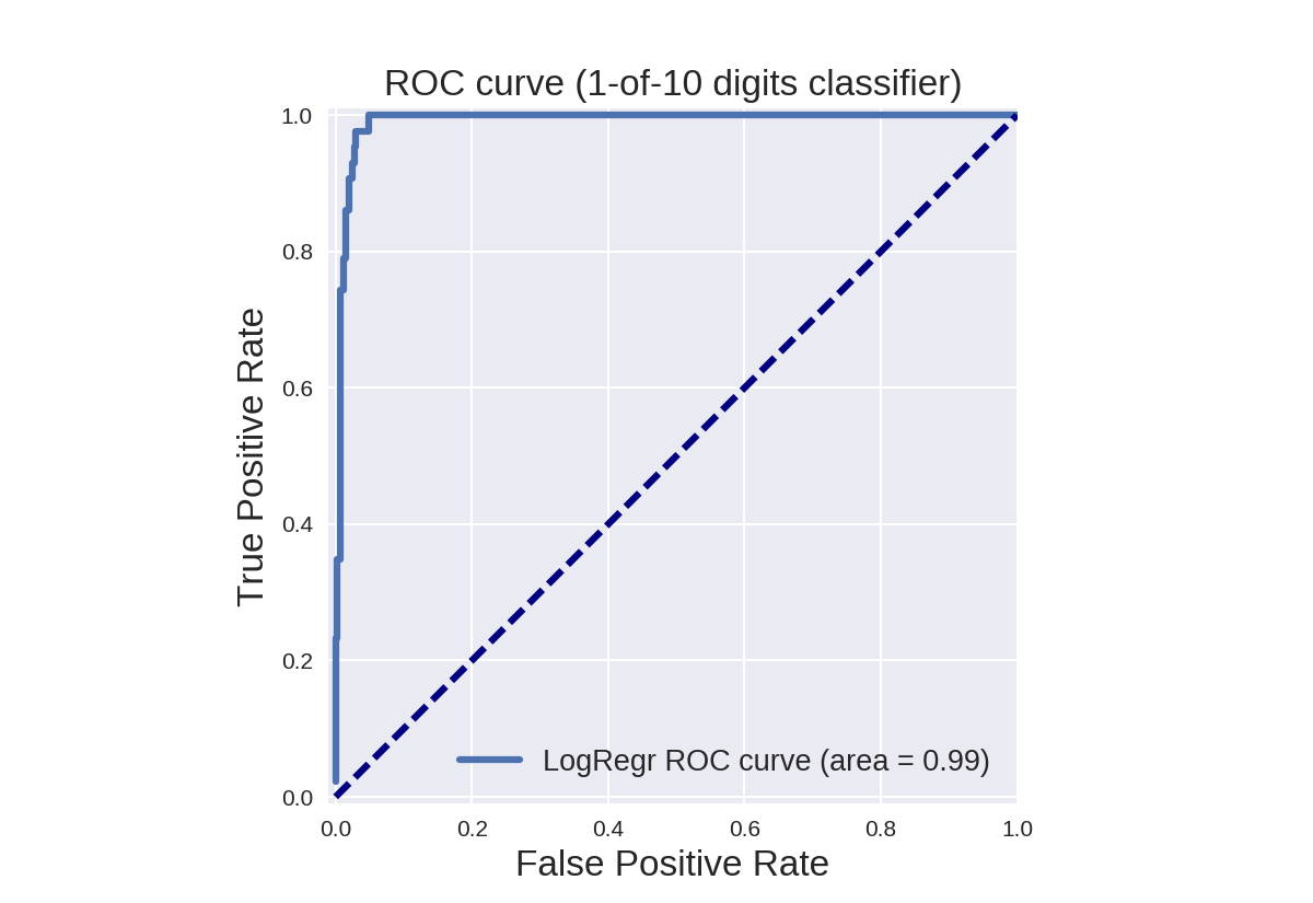
ROC curves, Area-Under-Curve (AUC)
 1 from sklearn.metrics import roc_curve, auc
 2
 3 X_train, X_test, y_train, y_test = train_test_split(X, y_binary_imbalanced, random_state=0)
 4
 5 y_score_lr = lr.fit(X_train, y_train).decision_function(X_test)
 6 fpr_lr, tpr_lr, _ = roc_curve(y_test, y_score_lr)
 7 roc_auc_lr = auc(fpr_lr, tpr_lr)
 8
 9 plt.figure()
10 plt.xlim([-0.01, 1.00])
11 plt.ylim([-0.01, 1.01])
12 plt.plot(fpr_lr, tpr_lr, lw=3, label='LogRegr ROC curve (area = {:0.2f})'.format(roc_auc_lr))
13 plt.xlabel('False Positive Rate', fontsize=16)
14 plt.ylabel('True Positive Rate', fontsize=16)
15 plt.title('ROC curve (1-of-10 digits classifier)', fontsize=16)
16 plt.legend(loc='lower right', fontsize=13)
17 plt.plot([0, 1], [0, 1], color='navy', lw=3, linestyle='--')
18 plt.axes().set_aspect('equal')
19 plt.show()
 1 from matplotlib import cm
 2
 3 X_train, X_test, y_train, y_test = train_test_split(X, y_binary_imbalanced, random_state=0)
 4
 5 plt.figure()
 6 plt.xlim([-0.01, 1.00])
 7 plt.ylim([-0.01, 1.01])
 8 for g in [0.01, 0.1, 0.20, 1]:
 9     svm = SVC(gamma=g).fit(X_train, y_train)
10     y_score_svm = svm.decision_function(X_test)
11     fpr_svm, tpr_svm, _ = roc_curve(y_test, y_score_svm)
12     roc_auc_svm = auc(fpr_svm, tpr_svm)
13     accuracy_svm = svm.score(X_test, y_test)
14     print("gamma = {:.2f}  accuracy = {:.2f}   AUC = {:.2f}".format(g, accuracy_svm,
15                                                                     roc_auc_svm))
16     plt.plot(fpr_svm, tpr_svm, lw=3, alpha=0.7,
17              label='SVM (gamma = {:0.2f}, area = {:0.2f})'.format(g, roc_auc_svm))
18
19 plt.xlabel('False Positive Rate', fontsize=16)
20 plt.ylabel('True Positive Rate (Recall)', fontsize=16)
21 plt.plot([0, 1], [0, 1], color='k', lw=0.5, linestyle='--')
22 plt.legend(loc="lower right", fontsize=11)
23 plt.title('ROC curve: (1-of-10 digits classifier)', fontsize=16)
24 plt.axes().set_aspect('equal')
25
26 plt.show()

对多分类模型的验证方法
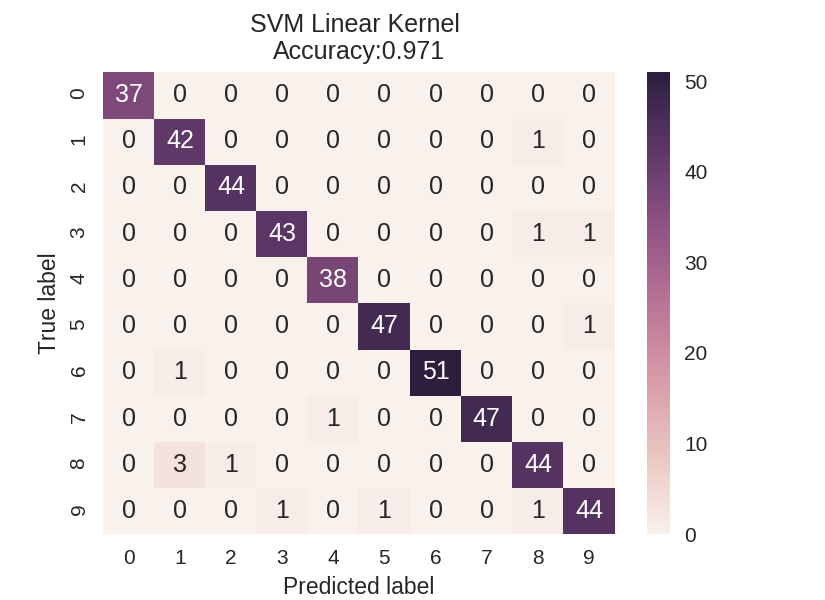
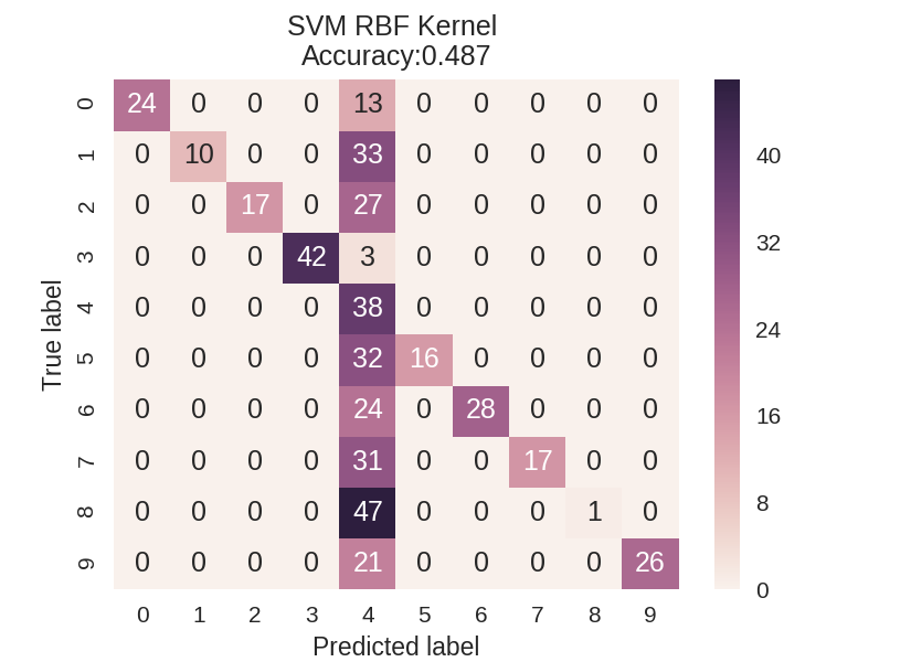
多分类模型的混淆矩阵
 1 dataset = load_digits()
 2 X, y = dataset.data, dataset.target
 3 X_train_mc, X_test_mc, y_train_mc, y_test_mc = train_test_split(X, y, random_state=0)
 4
 5
 6 svm = SVC(kernel = 'linear').fit(X_train_mc, y_train_mc)
 7 svm_predicted_mc = svm.predict(X_test_mc)
 8 confusion_mc = confusion_matrix(y_test_mc, svm_predicted_mc)
 9 df_cm = pd.DataFrame(confusion_mc,
10                      index = [i for i in range(0,10)], columns = [i for i in range(0,10)])
11
12 plt.figure(figsize=(5.5,4))
13 sns.heatmap(df_cm, annot=True)
14 plt.title('SVM Linear Kernel
Accuracy:{0:.3f}'.format(accuracy_score(y_test_mc,
15                                                                        svm_predicted_mc)))
16 plt.ylabel('True label')
17 plt.xlabel('Predicted label')
18
19
20 svm = SVC(kernel = 'rbf').fit(X_train_mc, y_train_mc)
21 svm_predicted_mc = svm.predict(X_test_mc)
22 confusion_mc = confusion_matrix(y_test_mc, svm_predicted_mc)
23 df_cm = pd.DataFrame(confusion_mc, index = [i for i in range(0,10)],
24                   columns = [i for i in range(0,10)])
25
26 plt.figure(figsize = (5.5,4))
27 sns.heatmap(df_cm, annot=True)
28 plt.title('SVM RBF Kernel
Accuracy:{0:.3f}'.format(accuracy_score(y_test_mc,
29                                                                     svm_predicted_mc)))
30 plt.ylabel('True label')
31 plt.xlabel('Predicted label');
多分类模型的报告
1 print(classification_report(y_test_mc, svm_predicted_mc))
             precision    recall  f1-score   support

          0       1.00      0.65      0.79        37
          1       1.00      0.23      0.38        43
          2       1.00      0.39      0.56        44
          3       1.00      0.93      0.97        45
          4       0.14      1.00      0.25        38
          5       1.00      0.33      0.50        48
          6       1.00      0.54      0.70        52
          7       1.00      0.35      0.52        48
          8       1.00      0.02      0.04        48
          9       1.00      0.55      0.71        47

avg / total       0.93      0.49      0.54       450
微观平均指标与宏观平均指标
1 print('Micro-averaged precision = {:.2f} (treat instances equally)'
2       .format(precision_score(y_test_mc, svm_predicted_mc, average = 'micro')))
3 print('Macro-averaged precision = {:.2f} (treat classes equally)'
4       .format(precision_score(y_test_mc, svm_predicted_mc, average = 'macro')))
Micro-averaged precision = 0.49 (treat instances equally)
Macro-averaged precision = 0.91 (treat classes equally)
1 print('Micro-averaged f1 = {:.2f} (treat instances equally)'
2       .format(f1_score(y_test_mc, svm_predicted_mc, average = 'micro')))
3 print('Macro-averaged f1 = {:.2f} (treat classes equally)'
4       .format(f1_score(y_test_mc, svm_predicted_mc, average = 'macro')))
Micro-averaged f1 = 0.49 (treat instances equally)
Macro-averaged f1 = 0.54 (treat classes equally)
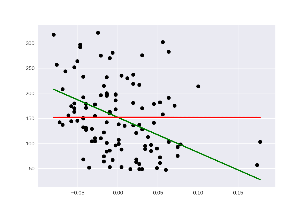
回归模型评估指标
 1 %matplotlib notebook
 2 import matplotlib.pyplot as plt
 3 import numpy as np
 4 from sklearn.model_selection import train_test_split
 5 from sklearn import datasets
 6 from sklearn.linear_model import LinearRegression
 7 from sklearn.metrics import mean_squared_error, r2_score
 8 from sklearn.dummy import DummyRegressor
 9
10 diabetes = datasets.load_diabetes()
11
12 X = diabetes.data[:, None, 6]
13 y = diabetes.target
14
15 X_train, X_test, y_train, y_test = train_test_split(X, y, random_state=0)
16
17 lm = LinearRegression().fit(X_train, y_train)
18 lm_dummy_mean = DummyRegressor(strategy = 'mean').fit(X_train, y_train)
19
20 y_predict = lm.predict(X_test)
21 y_predict_dummy_mean = lm_dummy_mean.predict(X_test)
22
23 print('Linear model, coefficients: ', lm.coef_)
24 print("Mean squared error (dummy): {:.2f}".format(mean_squared_error(y_test,
25                                                                      y_predict_dummy_mean)))
26 print("Mean squared error (linear model): {:.2f}".format(mean_squared_error(y_test, y_predict)))
27 print("r2_score (dummy): {:.2f}".format(r2_score(y_test, y_predict_dummy_mean)))
28 print("r2_score (linear model): {:.2f}".format(r2_score(y_test, y_predict)))
29
30 # Plot outputs
31 plt.scatter(X_test, y_test,  color='black')
32 plt.plot(X_test, y_predict, color='green', linewidth=2)
33 plt.plot(X_test, y_predict_dummy_mean, color='red', linestyle = 'dashed',
34          linewidth=2, label = 'dummy')
35
36 plt.show()
Linear model, coefficients:  [-698.80206267]
Mean squared error (dummy): 4965.13
Mean squared error (linear model): 4646.74
r2_score (dummy): -0.00
r2_score (linear model): 0.06
使用评估指标进行模型选择
交叉验证例子
 1 from sklearn.model_selection import cross_val_score
 2 from sklearn.svm import SVC
 3
 4 dataset = load_digits()
 5 # again, making this a binary problem with 'digit 1' as positive class
 6 # and 'not 1' as negative class
 7 X, y = dataset.data, dataset.target == 1
 8 clf = SVC(kernel='linear', C=1)
 9
10 # accuracy is the default scoring metric
11 print('Cross-validation (accuracy)', cross_val_score(clf, X, y, cv=5))
12 # use AUC as scoring metric
13 print('Cross-validation (AUC)', cross_val_score(clf, X, y, cv=5, scoring = 'roc_auc'))
14 # use recall as scoring metric
15 print('Cross-validation (recall)', cross_val_score(clf, X, y, cv=5, scoring = 'recall'))
Cross-validation (accuracy) [ 0.91944444  0.98611111  0.97214485  0.97493036  0.96935933]
Cross-validation (AUC) [ 0.9641871   0.9976571   0.99372205  0.99699002  0.98675611]
Cross-validation (recall) [ 0.81081081  0.89189189  0.83333333  0.83333333  0.83333333]
网格搜索示例
 1 from sklearn.svm import SVC
 2 from sklearn.model_selection import GridSearchCV
 3 from sklearn.metrics import roc_auc_score
 4
 5 dataset = load_digits()
 6 X, y = dataset.data, dataset.target == 1
 7 X_train, X_test, y_train, y_test = train_test_split(X, y, random_state=0)
 8
 9 clf = SVC(kernel='rbf')
10 grid_values = {'gamma': [0.001, 0.01, 0.05, 0.1, 1, 10, 100]}
11
12 # default metric to optimize over grid parameters: accuracy
13 grid_clf_acc = GridSearchCV(clf, param_grid = grid_values)
14 grid_clf_acc.fit(X_train, y_train)
15 y_decision_fn_scores_acc = grid_clf_acc.decision_function(X_test)
16
17 print('Grid best parameter (max. accuracy): ', grid_clf_acc.best_params_)
18 print('Grid best score (accuracy): ', grid_clf_acc.best_score_)
19
20 # alternative metric to optimize over grid parameters: AUC
21 grid_clf_auc = GridSearchCV(clf, param_grid = grid_values, scoring = 'roc_auc')
22 grid_clf_auc.fit(X_train, y_train)
23 y_decision_fn_scores_auc = grid_clf_auc.decision_function(X_test)
24
25 print('Test set AUC: ', roc_auc_score(y_test, y_decision_fn_scores_auc))
26 print('Grid best parameter (max. AUC): ', grid_clf_auc.best_params_)
27 print('Grid best score (AUC): ', grid_clf_auc.best_score_)
Grid best parameter (max. accuracy):  {'gamma': 0.001}
Grid best score (accuracy):  0.996288047513
Test set AUC:  0.999828581224
Grid best parameter (max. AUC):  {'gamma': 0.001}
Grid best score (AUC):  0.99987412783
1 #Evaluation metrics supported for model selection
2 from sklearn.metrics.scorer import SCORERS
3
4 print(sorted(list(SCORERS.keys())))
['accuracy', 'adjusted_rand_score', 'average_precision', 'f1', 'f1_macro', 'f1_micro',
'f1_samples', 'f1_weighted', 'log_loss', 'mean_absolute_error', 'mean_squared_error',
'median_absolute_error', 'neg_log_loss', 'neg_mean_absolute_error', 'neg_mean_square
d_error', 'neg_median_absolute_error', 'precision', 'precision_macro', 'precision_mic
ro', 'precision_samples', 'precision_weighted', 'r2', 'recall', 'recall_macro',
'recall_micro', 'recall_samples', 'recall_weighted', 'roc_auc']
使用数字数据集的双特征分类示例
使用不同的评估指标优化分类器
 1 from sklearn.datasets import load_digits
 2 from sklearn.model_selection import train_test_split
 3 from adspy_shared_utilities import plot_class_regions_for_classifier_subplot
 4 from sklearn.svm import SVC
 5 from sklearn.model_selection import GridSearchCV
 6
 7
 8 dataset = load_digits()
 9 X, y = dataset.data, dataset.target == 1
10 X_train, X_test, y_train, y_test = train_test_split(X, y, random_state=0)
11
12 # Create a two-feature input vector matching the example plot above
13 # We jitter the points (add a small amount of random noise) in case there are areas
14 # in feature space where many instances have the same features.
15 jitter_delta = 0.25
16 X_twovar_train = X_train[:,[20,59]]+ np.random.rand(X_train.shape[0], 2) - jitter_delta
17 X_twovar_test  = X_test[:,[20,59]] + np.random.rand(X_test.shape[0], 2) - jitter_delta
18
19 clf = SVC(kernel = 'linear').fit(X_twovar_train, y_train)
20 grid_values = {'class_weight':['balanced', {1:2},{1:3},{1:4},{1:5},{1:10},{1:20},{1:50}]}
21 plt.figure(figsize=(9,6))
22 for i, eval_metric in enumerate(('precision','recall', 'f1','roc_auc')):
23     grid_clf_custom = GridSearchCV(clf, param_grid=grid_values, scoring=eval_metric)
24     grid_clf_custom.fit(X_twovar_train, y_train)
25     print('Grid best parameter (max. {0}): {1}'
26           .format(eval_metric, grid_clf_custom.best_params_))
27     print('Grid best score ({0}): {1}'
28           .format(eval_metric, grid_clf_custom.best_score_))
29     plt.subplots_adjust(wspace=0.3, hspace=0.3)
30     plot_class_regions_for_classifier_subplot(grid_clf_custom, X_twovar_test, y_test, None,
31                                              None, None,  plt.subplot(2, 2, i+1))
32
33     plt.title(eval_metric+'-oriented SVC')
34 plt.tight_layout()
35 plt.show()

Grid best parameter (max. precision): {'class_weight': {1: 2}}
Grid best score (precision): 0.5379994354058584
Grid best parameter (max. recall): {'class_weight': {1: 50}}
Grid best score (recall): 0.921184706893106
Grid best parameter (max. f1): {'class_weight': {1: 3}}
Grid best score (f1): 0.5079935126308859
Grid best parameter (max. roc_auc): {'class_weight': {1: 20}}
Grid best score (roc_auc): 0.8889416320163174
默认SVC分类器的精确召回曲线(平衡类别权重)
 1 from sklearn.model_selection import train_test_split
 2 from sklearn.metrics import precision_recall_curve
 3 from adspy_shared_utilities import plot_class_regions_for_classifier
 4 from sklearn.svm import SVC
 5
 6 dataset = load_digits()
 7 X, y = dataset.data, dataset.target == 1
 8 X_train, X_test, y_train, y_test = train_test_split(X, y, random_state=0)
 9
10 # create a two-feature input vector matching the example plot above
11 jitter_delta = 0.25
12 X_twovar_train = X_train[:,[20,59]]+ np.random.rand(X_train.shape[0], 2) - jitter_delta
13 X_twovar_test  = X_test[:,[20,59]] + np.random.rand(X_test.shape[0], 2) - jitter_delta
14
15 clf = SVC(kernel='linear', class_weight='balanced').fit(X_twovar_train, y_train)
16
17 y_scores = clf.decision_function(X_twovar_test)
18
19 precision, recall, thresholds = precision_recall_curve(y_test, y_scores)
20 closest_zero = np.argmin(np.abs(thresholds))
21 closest_zero_p = precision[closest_zero]
22 closest_zero_r = recall[closest_zero]
23
24 plot_class_regions_for_classifier(clf, X_twovar_test, y_test)
25 plt.title("SVC, class_weight = 'balanced', optimized for accuracy")
26 plt.show()
27
28 plt.figure()
29 plt.xlim([0.0, 1.01])
30 plt.ylim([0.0, 1.01])
31 plt.title ("Precision-recall curve: SVC, class_weight = 'balanced'")
32 plt.plot(precision, recall, label = 'Precision-Recall Curve')
33 plt.plot(closest_zero_p, closest_zero_r, 'o', markersize=12, fillstyle='none', c='r', mew=3)
34 plt.xlabel('Precision', fontsize=16)
35 plt.ylabel('Recall', fontsize=16)
36 plt.axes().set_aspect('equal')
37 plt.show()
38 print('At zero threshold, precision: {:.2f}, recall: {:.2f}'
39       .format(closest_zero_p, closest_zero_r))
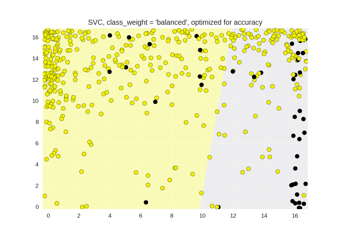
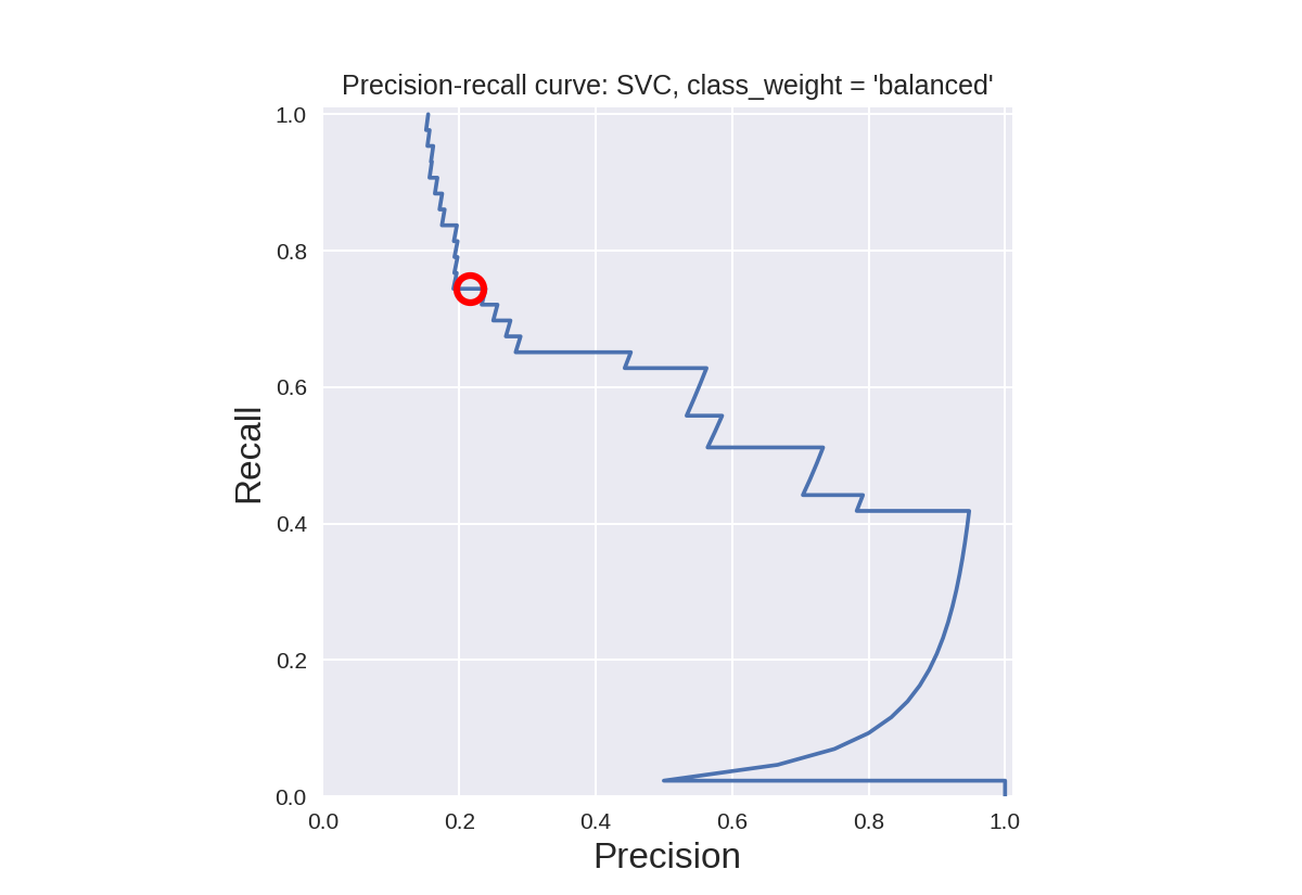
At zero threshold, precision: 0.22, recall: 0.74