一、介绍
二、编程
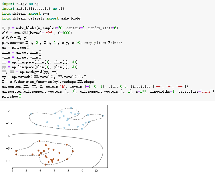
1、支持向量机的核函数
import numpy as np
import matplotlib.pyplot as plt
from sklearn import svm
from sklearn.datasets import make_blobs
X, y = make_blobs(n_samples=50, centers=2, random_state=6)
clf = svm.SVC(kernel='rbf', C=1000)
clf.fit(X, y)
plt.scatter(X[:, 0], X[:, 1], c=y, s=30, cmap=plt.cm.Paired)
ax = plt.gca()
xlim = ax.get_xlim()
ylim = ax.get_ylim()
xx = np.linspace(xlim[0], xlim[1], 30)
yy = np.linspace(ylim[0], ylim[1], 30)
YY, XX = np.meshgrid(yy, xx)
xy = np.vstack([XX.ravel(), YY.ravel()]).T
Z = clf.decision_function(xy).reshape(XX.shape)
ax.contour(XX, YY, Z, colors='k', levels=[-1, 0, 1], alpha=0.5, linestyles=['--', '-', '--'])
ax.scatter(clf.support_vectors_[:, 0], clf.support_vectors_[:, 1], s=100, linewidths=1, facecolors='none')
plt.show()
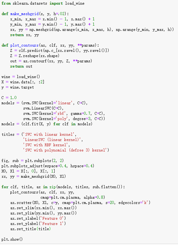
2、不同核函数的SVM对比
from sklearn.datasets import load_wine
def make_meshgrid(x, y, h=.02):
x_min, x_max = x.min() - 1, x.max() + 1
y_min, y_max = y.min() - 1, y.max() + 1
xx, yy = np.meshgrid(np.arange(x_min, x_max, h), np.arange(y_min, y_max, h))
return xx, yy
def plot_contours(ax, clf, xx, yy, **params):
Z = clf.predict(np.c_[xx.ravel(), yy.ravel()])
Z = Z.reshape(xx.shape)
out = ax.contourf(xx, yy, Z, **params)
return out
wine = load_wine()
X = wine.data[:, :2]
y = wine.target
C = 1.0
models = (svm.SVC(kernel='linear', C=C),
svm.LinearSVC(C=C),
svm.SVC(kernel='rbf', gamma=0.7, C=C),
svm.SVC(kernel='poly', degree=3, C=C))
models = (clf.fit(X, y) for clf in models)
titles = ('SVC with linear kernel',
'LinearSVC (linear kernel)',
'SVC with RBF kernel',
'SVC with polynomial (defree 3) kernel')
fig, sub = plt.subplots(2, 2)
plt.subplots_adjust(wspace=0.4, hspace=0.4)
X0, X1 = X[:, 0], X[:, 1]
xx, yy = make_meshgrid(X0, X1)
for clf, title, ax in zip(models, titles, sub.flatten()):
plot_contours(ax, clf, xx, yy,
cmap=plt.cm.plasma, alpha=0.8)
ax.scatter(X0, X1, c=y, cmap=plt.cm.plasma, s=20, edgecolors='k')
ax.set_xlim(xx.min(), xx.max())
ax.set_ylim(yy.min(), yy.max())
ax.set_xlabel('Feature 0')
ax.set_ylabel('Feature 1')
ax.set_title(title)
plt.show()

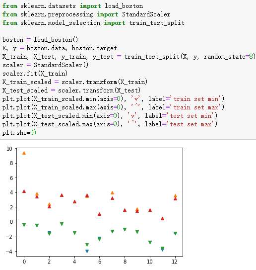
3、SVM实例-波士顿房价回归分析
from sklearn.datasets import load_boston
from sklearn.preprocessing import StandardScaler
from sklearn.model_selection import train_test_split
boston = load_boston()
X, y = boston.data, boston.target
X_train, X_test, y_train, y_test = train_test_split(X, y, random_state=8)
scaler = StandardScaler()
scaler.fit(X_train)
X_train_scaled = scaler.transform(X_train)
X_test_scaled = scaler.transform(X_test)
plt.plot(X_train_scaled.min(axis=0), 'v', label='train set min')
plt.plot(X_train_scaled.max(axis=0), '^', label='train set max')
plt.plot(X_test_scaled.min(axis=0), 'v', label='test set min')
plt.plot(X_test_scaled.max(axis=0), '^', label='test set max')
plt.show()