当我们面对一个非线性的ODE时,我们要怎么解决它?
推荐看这篇介绍文章:http://www.phys.uconn.edu/~rozman/Courses/P2400_15S/downloads/averaging.pdf
这里写下我的理解:
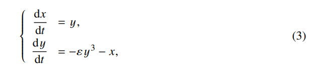
以一个单自由度的mass-damper-spring系统为例,但是这里的阻尼不是关于速度线性的,而是关于速度的三次非线性的,其控制方程和初始条件如下所示:


1. 首先用数值方法得到数值解作为对比,将二阶的ODE写成两个一阶的ODEs:
该ODEs可以直接用Matlab的ode45求解,代码如下:
% numerical solution by ode45
epsilon = 0.2;
tspan = 0:0.01:50;
y0 = [1; 0];
[~, y] = ode45(@(t,y) equations(y, epsilon), tspan, y0);
%  each row in y corresponds to the solution at the value returned
%  in the corresponding row of t.
plot(tspan, y(:,1),'linewidth',1.5)
grid on

function dydt = equations(y, epsilon)
% oscillator with nonlinear friction
% y(1) ---> x
% y(2) ---> dx/dt
y = y(:);
dydt = zeros(size(y));
dydt(1) = y(2);
dydt(2) = -epsilon*y(2)^3-y(1);
end
结果如下图:
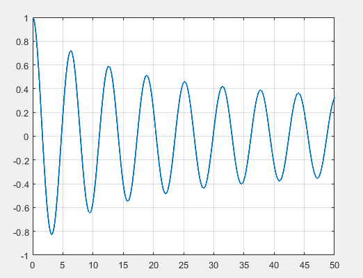
表示位移x(t)随时间的变化
2.用摄动法(perturbation)求近似解析解
首先将x(t)按epsilon的幂次展开

(为什么要这样展开?我的理解:把解分成几部分之和,每一部分的幅值大小由epsilon刻画,因为epsilon是一个小量,显然x0(t)对x(t)的贡献最主要,x1(t)次之,贡献依次递减。也就是说认为x(t)主要是按x(t)变化,受到了一些摄动x1(t),摄动x1(t)对x(t)的影响大小与小量epsilon同阶。这种展开应该主要应用在弱非线性的系统,即认为解x(t)仍然主要按对应线性系统的解x0(t)变化,再加上一点非线性的影响(摄动)x1(t),x2(t),这些摄动的影响是小量的。因为是从小量epsilon对解的影响来看待问题的,所以这种方法主要适用于弱非线性系统)
按这种方式展开之后,为了与原初始条件协调一致,这些分量的初始条件应该为

将展开式(5)式代入原方程(1)式,并让同一epsilon的幂次的合并,可以得到一系列线性的方程,注意看到由于非线性(这里是三次方)的存在,展开的时候显然很麻烦,这也是摄动法的一个缺点
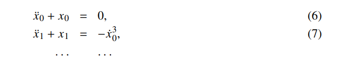
这里只写到epsilon的一次项,一般来说对于近似解这就足够的,而且更高次的写出来显然很麻烦
注意到第一个方程,x0,是线性的,其对x的贡献是epsilon的零次的,也就是最主要的,接下来epsilon的一次幂的解x1对x的贡献与epsilon的一次同阶,表示摄动。在下面的分析中我们这考虑x1,其他摄动量都是很小的(其大小程度由epsilon的幂次衡量)
线性部分(主要部分)的满足初始条件的解是

对于epsilon的一阶项,注意到x0已经求出来了,所以是线性的方程。也就是说用摄动法我们可以得到对每一个epsilon的幂次的线性方程,这是摄动法的优点,把非线性方程分成几个线性的方程求解。但是要注意到等式右边一般来说是关于时间t的复杂的表达式(一般是三角函数),所以即使是要求解一个线性微分方程的解析解也是麻烦的
以(7)式子为例,
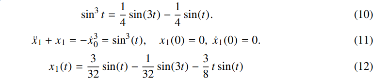
至此我们可以得到一个近似的解析解:

将该结果与上面用ode45得到的数值解作对比
代码如下
% numerical solution by ode45
epsilon = 0.2;
tspan = 0:0.01:50;
y0 = [1; 0];
[~, y] = ode45(@(t,y) equations(y, epsilon), tspan, y0);
%  each row in y corresponds to the solution at the value returned
%  in the corresponding row of t.
plot(tspan, y(:,1),'b','linewidth',1.5)
grid on
hold on
% perturbation solution
x1 = cos(tspan)+epsilon*(3/32*sin(tspan)-1/32*sin(3*tspan)-3/8*tspan.*sin(tspan));
plot(tspan,x1, 'r', 'linewidth', 1.5)

legend('ode45(benchmark)','perturbation')


function dydt = equations(y, epsilon)
% oscillator with nonlinear friction
% y(1) ---> x
% y(2) ---> dx/dt
y = y(:);
dydt = zeros(size(y));
dydt(1) = y(2);
dydt(2) = -epsilon*y(2)^3-y(1);
end
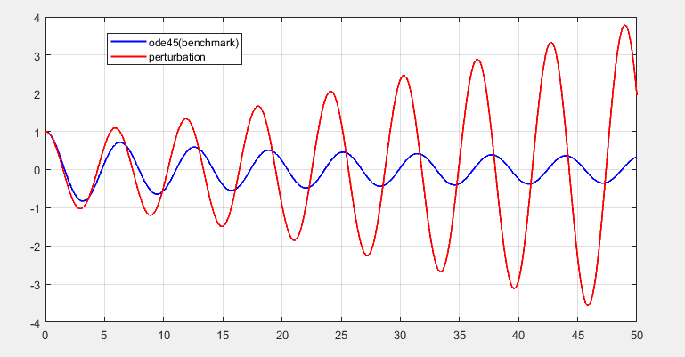
可见摄动法的解只有在开始的一段很短的时间是对的,很快后面就不对了,会发散(变得很大)。所以摄动法是有问题的。问题出现在什么地方?让我们看一下用摄动法得到的解
显然是由于 这一项的存在才会使得解会发散(grow undounded as t increases),这一项叫做长期项(secular term)。虽然一般翻译成长期项,但是我想英文想表达的是(not bound by monastic vows or rules)的意思,(翻译成病态项或许更好?),而不是长期存在,因为别的项也长期存在(比如sin(t), sin(3t)),所以接下里不用长期项这种翻译而是直接用secular term
secular term之所以会出现是因为在(11)式的右边(激励)有 这一部分,注意到其激励频率等于左边系统的固有频率,即发生了共振。
这是摄动法的一个常见缺点(或者说致命缺点?),至于为什么会出现,什么情况下可以避免,这里暂时不深入。总之只需要知道摄动法求解时有时候会由于(人为地引入)共振的出现,导致解有secular term。
3. 平均法
平均法可以用来求解下面这一类关于一阶导数非线性的非线性ODE:
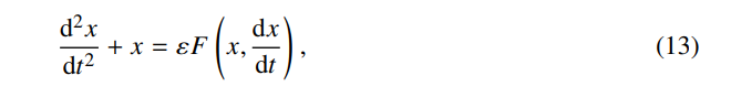
上一节用摄动法考虑的例子是一个特例: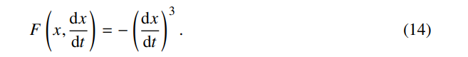
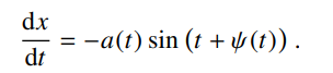
平均法考虑(13)式具有如下形式的解和速度解,注意不仅假设了位移的形式,同时也假设了速度具有和线性时相同的形式:

为什么要这么考虑?因为当非线性消失时,退化的线性ODE的解具有(15)式和(16)式的形式,不过此时的幅值和相位是由初始条件决定的常数;当系统有了一点弱非线性时,我们可以乐观地假设方程的解仍然具有(15)式的形式,不过此时幅值和相位是会随时间变化的函数,并且认为幅值和相位是缓慢变化的。为什么认为是缓慢变化的?因为缓慢变化的话方程的解才大致地具有和线性时候的解一样的形式,只不过由于非线性带来幅值和相位的缓慢变化。注意这里频率仍然是固定的。若非线性出现在会影响频率的刚度项,又该怎么做呢?
这是平均法的核心,或者说亮点吧,就是洞见问题的解具有(15)和(16)式的形式。
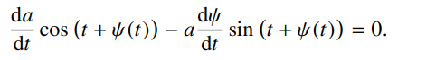
将(15)式求导代入(16)式得到一个方程,将(16)式求导代入(1)式,得到两个耦合的ODEs


整理成

到这一步为止都是精确的,不过是假设了解的形式,但没有作任何的近似或者截断。
接下来为了求解(20)和(21)式,要做一点假设:
因为是弱非线性,即epsilon是个小量,所以认为幅值和相位的变化是缓慢的,即幅值和相位的导数是小量。这样的话,在振动的一个周期内(这里频率是1,所以周期是2pi),(20)式和(21)式的方程右边几乎保持不变是一个常数,这样就可以用它们在一个周期内的平均作近似。(这样的近似还是不是很理解)

(20)和(21)式变为下面的形式,是平均化的方程

注意到积分后时间变量就消去了(消除快变量),(不是很理解)
对(23)式和(24)式右边的积分计算,需要用到三角恒等式
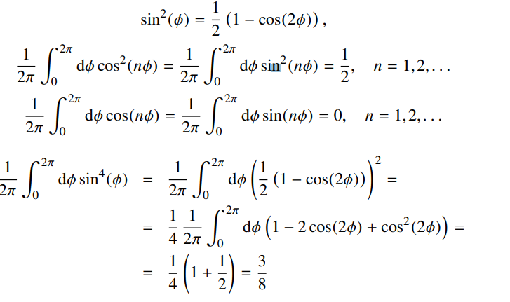
最终(23)和(24)式变为
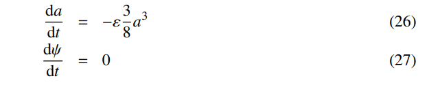
(26)式和(27)式可以较轻易地求解: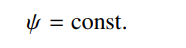


最终解为下面的形式,其中a(0)由初始条件确定为x(0)

和数值解作比较发现是较为精确地!而且和数值解相比具有解析形式的优势。

代码如下:
% numerical solution by ode45
epsilon = 0.2;
tspan = 0:0.01:50;
y0 = [1; 0];
[~, y] = ode45(@(t,y) equations(y, epsilon), tspan, y0);
%  each row in y corresponds to the solution at the value returned
%  in the corresponding row of t.
plot(tspan, y(:,1),'b','linewidth',2)
grid on
hold on
% perturbation solution
x1 = cos(tspan)+epsilon*(3/32*sin(tspan)-1/32*sin(3*tspan)-3/8*tspan.*sin(tspan));
plot(tspan,x1, 'r', 'linewidth', 1.5)
% averaged solution
x2 = cos(tspan)./sqrt(3/4*epsilon*tspan+1/1^2);
plot(tspan,x2,'y--')
legend('ode45(benchmark)','perturbation','averaged')


function dydt = equations(y, epsilon)
% oscillator with nonlinear friction
% y(1) ---> x
% y(2) ---> dx/dt
y = y(:);
dydt = zeros(size(y));
dydt(1) = y(2);
dydt(2) = -epsilon*y(2)^3-y(1);
end
4. 接下来考虑另一个系统,这是一个著名的非线性系统,叫做van der pol振子,具有(13)式的形式,因此也可以用平均法求近似解析解

求数值解(ode45)时仍然要先转化为一阶的ODEs

求近似解析解时,和上面一样的思路和步骤,首先假设解的形式为:
第一式求导代入第二式,第二式求导代入方程,得到

整理:
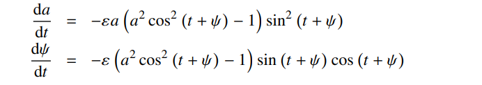
接下来做平均:

计算积分同样要用到三角恒等式
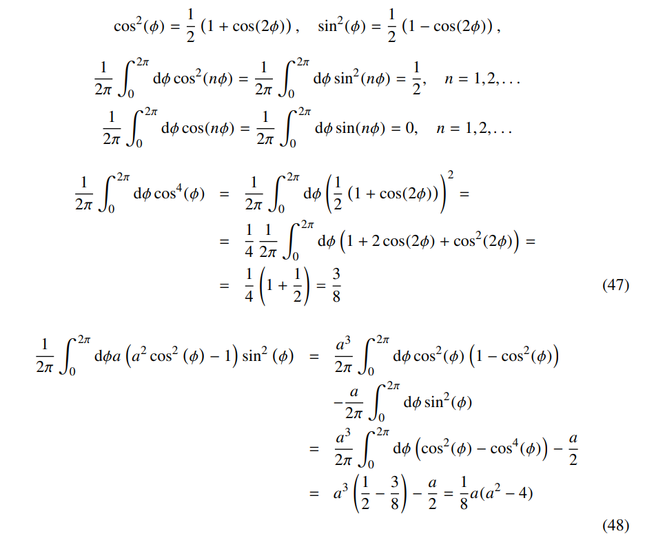
最后得到
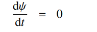

求解ODE(实际还很难求解的):


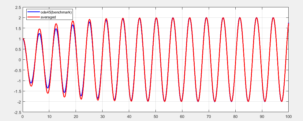
和数值解作比较,在前面一段时间有点误差,后面对得还好:
代码如下
% numerical solution by ode45
epsilon = 0.1;
tspan = 0:0.01:100;
y0 = [1; 0];
[~, y] = ode45(@(t,y) equations(y, epsilon), tspan, y0);
%  each row in y corresponds to the solution at the value returned
%  in the corresponding row of t.
plot(tspan, y(:,1),'b','linewidth',2)
grid on
hold on
% averaged solution
x2 = (2-exp(-epsilon*tspan)).*cos(tspan);
plot(tspan,x2,'r','linewidth',2)
legend('ode45(benchmark)','averaged')


function dydt = equations(y, epsilon)
% oscillator with nonlinear friction
% y(1) ---> x
% y(2) ---> dx/dt
y = y(:);
dydt = zeros(size(y));
dydt(1) = y(2);
dydt(2) = -epsilon*(y(1)^2-1)*y(2)-y(1);
end
总结:
平均法的两个步骤:
一是假设解的形式,这个形式由非线性激励和/或非线性阻尼中的小参数取零时确定,即系统在无阻尼无激励时的精确解形式,然后令幅值和相位变为时间的函数
二是认为幅值和相位的变化是小量,在一个周期内不变,所以可以对时间在一个周期上上作平均,去掉快变量
练习:
1.Duffing

我的解答: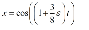

代码如下
% numerical solution by ode45
epsilon = 0.2;
tspan = 0:0.01:25;
y0 = [1; 0];
[~, y] = ode45(@(t,y) equations(y, epsilon), tspan, y0);
%  each row in y corresponds to the solution at the value returned
%  in the corresponding row of t.
plot(tspan, y(:,1),'b','linewidth',2)
grid on
hold on
% averaged solution
x2 = cos((1+3/8*epsilon)*tspan);
plot(tspan,x2,'r','linewidth',2)
legend('ode45(benchmark)','averaged')


function dydt = equations(y, epsilon)
% oscillator with nonlinear friction
% y(1) ---> x
% y(2) ---> dx/dt
y = y(:);
dydt = zeros(size(y));
dydt(1) = y(2);
dydt(2) = -epsilon*y(1)^3-y(1);
end
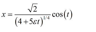
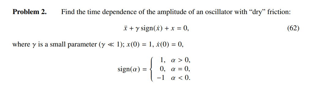
3.

我的解答
数值解对比

代码:
% numerical solution by ode45
epsilon = 0.03;
tspan = 0:0.01:25;
y0 = [1; 0];
[~, y] = ode45(@(t,y) equations(y, epsilon), tspan, y0);
%  each row in y corresponds to the solution at the value returned
%  in the corresponding row of t.
plot(tspan, y(:,1),'b','linewidth',3)
grid on
hold on
% averaged solution
x2 = sqrt(2)./(4+5*epsilon*tspan).^(1/4).*cos(tspan);
plot(tspan,x2,'r','linewidth',1.5)
legend('ode45(benchmark)','averaged')


function dydt = equations(y, epsilon)
% oscillator with nonlinear friction
% y(1) ---> x
% y(2) ---> dx/dt
y = y(:);
dydt = zeros(size(y));
dydt(1) = y(2);
dydt(2) = -epsilon*y(2)^5-y(1);
end
2.
看起来有点麻烦,罢了
后续应对平均法作深入了解,是求解非线性微分方程的近似解析解的主要方法