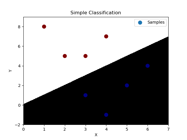
'''
    逻辑分类:----底层为线性回归问题
        通过输入的样本数据,基于多元线型回归模型求出线性预测方程。
            y = w0+w1x1+w2x2
        但通过线型回归方程返回的是连续值,不可以直接用于分类业务模型,所以急需一种方式使得把连续的预测值->离散的预测值。
         [-oo, +oo]->{0, 1}
         逻辑函数(sigmoid):y = 1 / (1+e^(-x)), 该逻辑函数当x>0,y>0.5;当x<0, y<0.5;
        可以把样本数据经过线性预测模型求得的值带入逻辑函数的x,即将预测函数的输出看做输入被划分为1类的概率,
        择概率大的类别作为预测结果,可以根据函数值确定两个分类。这是连续函数离散化的一种方式。

    逻辑回归相关API:
            import sklearn.linear_model as lm
            # 构建逻辑回归器
            # solver:逻辑函数中指数的函数关系(liblinear为线型函数关系)
            # C:参数代表正则强度,为了防止过拟合。正则越大拟合效果越小。
            model = lm.LogisticRegression(solver='liblinear', C=正则强度)
            model.fit(训练输入集,训练输出集)
            result = model.predict(带预测输入集)

    案例:基于逻辑回归器绘制网格化坐标颜色矩阵。
'''
import numpy as np
import matplotlib.pyplot as mp
import sklearn.linear_model as lm

x = np.array([[3, 1],
              [2, 5],
              [1, 8],
              [6, 4],
              [5, 2],
              [3, 5],
              [4, 7],
              [4, -1]])
y = np.array([0, 1, 1, 0, 0, 1, 1, 0])
# 根据找到的某些规律,绘制分类边界线
l, r = x[:, 0].min() - 1, x[:, 0].max() + 1
b, t = x[:, 1].min() - 1, x[:, 1].max() + 1
n = 500
grid_x, grid_y = np.meshgrid(np.linspace(l, r, n), np.linspace(b, t, n))
# 构建逻辑回归模型,并训练模型
model = lm.LogisticRegression(solver='liblinear', C=1)
model.fit(x, y)
# 把网格坐标矩阵中500*500做类别预测
test_x = np.column_stack((grid_x.ravel(), grid_y.ravel()))      # grid_x,grid_y撑平后合并为两列
test_y = model.predict(test_x)
grid_z = test_y.reshape(grid_x.shape)

# 绘制样本数据
mp.figure('Simple Classification', facecolor='lightgray')
mp.title('Simple Classification')
mp.xlabel('X')
mp.ylabel('Y')
# 绘制分类边界线(填充网格化矩阵)
mp.pcolormesh(grid_x, grid_y, grid_z, cmap='gray')
mp.scatter(x[:, 0], x[:, 1], s=80, c=y, cmap='jet', label='Samples')

mp.legend()
mp.show()
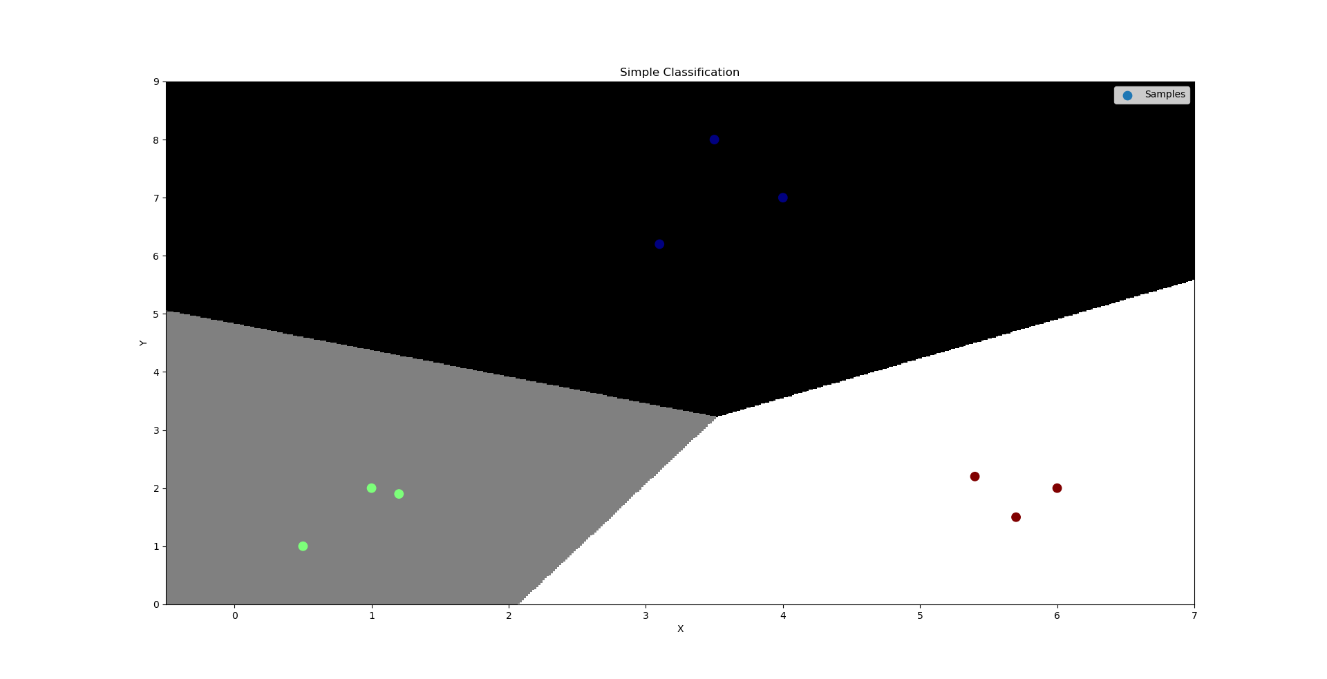
'''
    多元逻辑分类:----底层为线性回归问题
        通过多个二元分类器解决多元分类问题。
            特征1    特征2    ==>    所属类别
            4        7        ==>     A
            3.5        8        ==>        A
            1.2        1.9     ==>     B
            5.4        2.2     ==>     C
        若拿到一组新的样本,可以基于二元逻辑分类训练出一个模型判断属于A类别的概率。
        再使用同样的方法训练出两个模型分别判断属于B、C类型的概率,最终选择概率最高的类别作为新样本的分类结果。

    逻辑回归相关API:
            import sklearn.linear_model as lm
            # 构建逻辑回归器
            # solver:逻辑函数中指数的函数关系(liblinear为线型函数关系)
            # C:参数代表正则强度,为了防止过拟合。正则越大拟合效果越小。
            model = lm.LogisticRegression(solver='liblinear', C=正则强度)
            model.fit(训练输入集,训练输出集)
            result = model.predict(带预测输入集)

    案例:基于逻辑分类模型的多元分类。
'''
import numpy as np
import matplotlib.pyplot as mp
import sklearn.linear_model as lm

x = np.array([[4, 7],
              [3.5, 8],
              [3.1, 6.2],
              [0.5, 1],
              [1, 2],
              [1.2, 1.9],
              [6, 2],
              [5.7, 1.5],
              [5.4, 2.2]])
y = np.array([0, 0, 0, 1, 1, 1, 2, 2, 2])
# 根据找到的某些规律,绘制分类边界线
l, r = x[:, 0].min() - 1, x[:, 0].max() + 1
b, t = x[:, 1].min() - 1, x[:, 1].max() + 1
n = 500
grid_x, grid_y = np.meshgrid(np.linspace(l, r, n), np.linspace(b, t, n))
# 构建逻辑回归模型,并训练模型
model = lm.LogisticRegression(solver='liblinear', C=200)
model.fit(x, y)
# 把网格坐标矩阵中500*500做类别预测
test_x = np.column_stack((grid_x.ravel(), grid_y.ravel()))  # grid_x,grid_y撑平后合并为两列
test_y = model.predict(test_x)
grid_z = test_y.reshape(grid_x.shape)

# 绘制样本数据
mp.figure('Simple Classification', facecolor='lightgray')
mp.title('Simple Classification')
mp.xlabel('X')
mp.ylabel('Y')
# 绘制分类边界线(填充网格化矩阵)
mp.pcolormesh(grid_x, grid_y, grid_z, cmap='gray')
mp.scatter(x[:, 0], x[:, 1], s=80, c=y, cmap='jet', label='Samples')

mp.legend()
mp.show()