一、符号函数
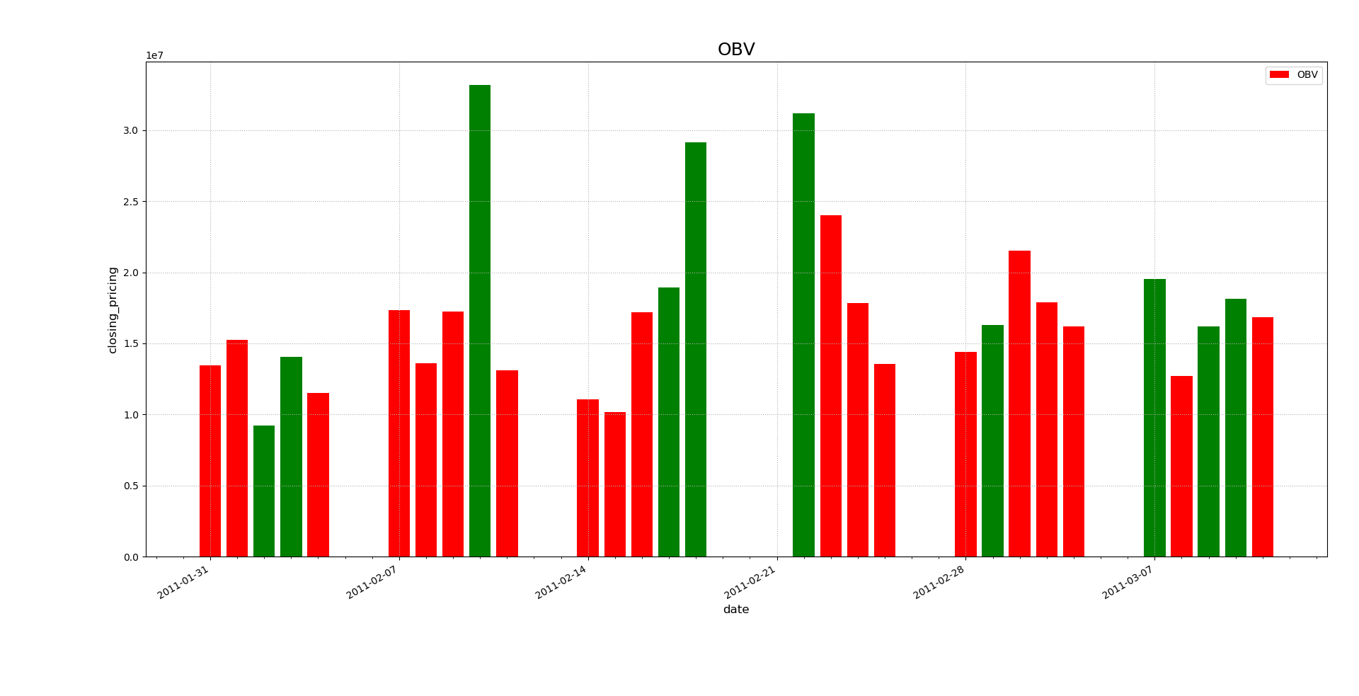
'''
    符号函数:np.sign(array)函数可以 把样本数组变成对应的符号数组,所有的证书变成1,负数变成-1,0还是0
            ----OBV能量潮(净额成交量)
'''
import numpy as np
import matplotlib.pyplot as mp
import datetime as dt
import matplotlib.dates as md


# 日期转化函数
def dmy2ymd(dmy):
    # 把dmy格式的字符串转化成ymd格式的字符串
    dmy = str(dmy, encoding='utf-8')
    d = dt.datetime.strptime(dmy, '%d-%m-%Y')
    d = d.date()
    ymd = d.strftime('%Y-%m-%d')
    return ymd


dates, opening_prices, highest_prices, lowest_prices, closing_prices, volumns =
    np.loadtxt('./da_data/aapl.csv', delimiter=',', usecols=(1, 3, 4, 5, 6, 7), unpack=True,
               dtype='M8[D], f8, f8, f8, f8, f8', converters={1: dmy2ymd})  # converters为转换器,运行时先执行,其中1表示时间所在的列索引号

# 绘制收盘价折线图
mp.figure('OBV', facecolor='lightgray')
mp.title('OBV', fontsize=18)
mp.xlabel('date', fontsize=12)
mp.ylabel('closing_pricing', fontsize=12)
mp.tick_params(labelsize=10)
mp.grid(linestyle=':')
# 设置x轴的刻度定位器,使之更适合显示日期数据
ax = mp.gca()
# 以周一作为主刻度
ma_loc = md.WeekdayLocator(byweekday=md.MO)
# 次刻度,除周一外的日期
mi_loc = md.DayLocator()
ax.xaxis.set_major_locator(ma_loc)
ax.xaxis.set_major_formatter(md.DateFormatter('%Y-%m-%d'))
ax.xaxis.set_minor_locator(mi_loc)
# 日期数据类型转换,更适合绘图
dates = dates.astype(md.datetime.datetime)
# 绘制OBV能量潮
# 若相比上一天的收盘价上涨,则为正成交量
# 若相比上一天的收盘价下跌,则为负成交量
diff_prices = np.diff(closing_prices)
sign_prices = np.sign(diff_prices)
obvs = volumns[1:]
color = [('red' if x == 1 else 'green') for x in sign_prices]
mp.bar(dates[1:], obvs, color=color, width=0.8, label='OBV')

mp.tight_layout()
mp.legend()
# 自动格式化x轴日期的显示格式(以最合适的方式显示)
mp.gcf().autofmt_xdate()
mp.show()
二、数组处理函数(符号函数的拓展)
'''
    数组处理函数:np.piecewise(原数组,条件序列,取值序列)
'''
import numpy as np

a = np.array([65, 78, 82, 99, 50])
# 数组处理,分类分数级别
r = np.piecewise(a, [a >= 85, (a >= 60) & (a < 85), a < 60], [1, 2, 3])
print(r)


输出结果:

    [2 2 2 1 3]
三、函数矢量化
'''
    函数矢量化:一般的函数只能处理标量参数,对该函数执行函数矢量化后,则会具备处理数组数据的能力
        ----numpy提供了vectorize函数和frompyfunc函数,可以把处理标量的函数矢量化,返回的函数可以直接接受矢量参数
        ----在传参的时候,如果全部传入数组,则数组维度要一致,此外,传参的时候也可以参入标量(数组每个元素与标量运算)
'''
import math as m
import numpy as np


def f(a, b):
    return m.sqrt(a ** 2 + b ** 2)


print(f(3, 4))
a = np.array([3, 4, 5, 6])
b = np.array([4, 5, 6, 7])
# 方法1:使用vectorize对函数矢量化,改造f函数,使之可以处理矢量数据
f_vec = np.vectorize(f)  # 返回矢量函数
print('第一次', f_vec(a, b))

print('第二次', np.vectorize(f)(a, b))

# 方法2:使用frompyfunc对函数矢量化
# 2:f函数接收2个参数
# 1:f函数有1个返回值
f_fpf = np.frompyfunc(f, 2, 1)
print('第三次', f_fpf(a, b))


输出结果:
    5.0
    第一次 [5.         6.40312424 7.81024968 9.21954446]
    第二次 [5.         6.40312424 7.81024968 9.21954446]
    第三次 [5.0 6.4031242374328485 7.810249675906654 9.219544457292887]
四、函数矢量化示例
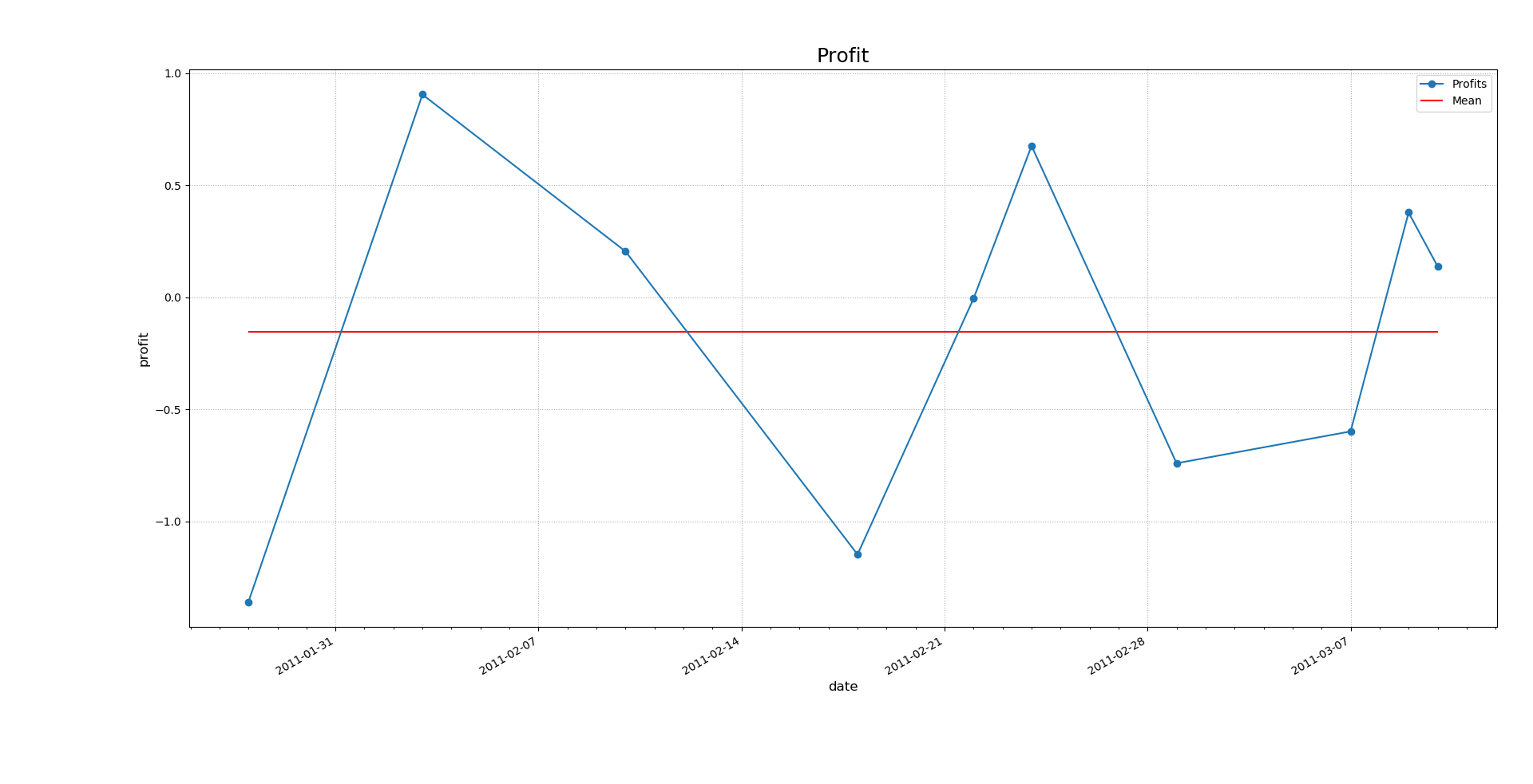
import numpy as np
import matplotlib.pyplot as mp
import datetime as dt
import matplotlib.dates as md

'''
    矢量化函数vectorize应用:计算收益策略是否合理---只要开盘价下降1%且在最高价和最低价之间就进行买入,收盘时卖出,否则不买
'''


# 日期转化函数
def dmy2ymd(dmy):
    # 把dmy格式的字符串转化成ymd格式的字符串
    dmy = str(dmy, encoding='utf-8')
    d = dt.datetime.strptime(dmy, '%d-%m-%Y')
    d = d.date()
    ymd = d.strftime('%Y-%m-%d')
    return ymd


dates, opening_prices, highest_prices, lowest_prices, closing_prices =
    np.loadtxt('./da_data/aapl.csv', delimiter=',', usecols=(1, 3, 4, 5, 6), unpack=True,
               dtype='M8[D], f8, f8, f8, f8', converters={1: dmy2ymd})  # converters为转换器,运行时先执行,其中1表示时间所在的列索引号

# 绘制收盘价折线图
mp.figure('Profit', facecolor='lightgray')
mp.title('Profit', fontsize=18)
mp.xlabel('date', fontsize=12)
mp.ylabel('profit', fontsize=12)
mp.tick_params(labelsize=10)
mp.grid(linestyle=':')
# 设置x轴的刻度定位器,使之更适合显示日期数据
ax = mp.gca()
# 以周一作为主刻度
ma_loc = md.WeekdayLocator(byweekday=md.MO)
# 次刻度,除周一外的日期
mi_loc = md.DayLocator()
ax.xaxis.set_major_locator(ma_loc)
ax.xaxis.set_major_formatter(md.DateFormatter('%Y-%m-%d'))
ax.xaxis.set_minor_locator(mi_loc)
# 日期数据类型转换,更适合绘图
dates = dates.astype(md.datetime.datetime)


def profit(opening_price, highest_price, lowest_price, closing_price):
    # 定义一种买入卖出策略
    buying_price = opening_price * 0.99
    if lowest_price <= buying_price <= highest_price:
        return (closing_price - buying_price) / buying_price * 100
    return np.nan


# 把profit函数矢量化,求得30天的交易数据
profits = np.vectorize(profit)(opening_prices, highest_prices, lowest_prices, closing_prices)
# 基于掩码,获取所有交易数据
nan = np.isnan(profits)
dates, profits = dates[~nan], profits[~nan]

mp.plot(dates, profits, 'o-', label='Profits')
mean = np.mean(profits)
mp.hlines(mean, dates[0], dates[-1], colors='red', label='Mean')

mp.tight_layout()
mp.legend()
# 自动格式化x轴日期的显示格式(以最合适的方式显示)
mp.gcf().autofmt_xdate()
mp.show()
五、numpy通用函数
'''
    数组的通用函数:
        1.ndarray.clip(min=下限,max=上限):裁剪函数,将数组中小于下限值或者大于上限值的元素值修改为下限值或者上限值
        2.ndarray.compress:压缩函数,类似掩码,即将符合条件的数组元素筛选出来
        3.np.all([条件1,条件2],axis=0),筛选函数(与的关系),将数组按照列方向,同时符合条件1和条件2的元素筛选出来
        4.np.any([条件1,条件2],axis=0),筛选函数(或的关系),将数组按照列方向,符合条件1或者条件2的元素筛选出来
        5.np.add(a,b):数组a,b对应元素的和
        6.np.add.reduce(a):数组a的所有元素的累加和
        7.np.add.accumulate(a):数组a的所有元素的累加和的过程
        8.np.add.outer([10,20,30],a):外和
        9.np.prod(a):数组a的所有元素累乘
        10.np.cumprod(a):数组a所有元素累乘的过程
        11.np.outer([10,20,30],a):外积
        12.np.divide(a,b):等价a/b
        13.np.floor_divide(a,b):地板除
        14.np.ceil(a):天花板除
        15.np.round(a):四舍五入
        16.np.trunc(a):截断取整
        17.np.bitwise_xor(a,b)<==>a^b :位异或(相同则0,相异则1)
        18.np.bitwise_and(a,b):按位与(必须两个都为1)
        19.np.bitwise_or(a,b):按位或 (只要有一个为1,则为1)
        20.np.bitwise_not(a):取反
        21.np.left_shift(a,2):左移
        22.np.right_shift(a,2):右移


'''
import numpy as np

a = np.arange(1, 11)
print(a.clip(min=4, max=8))
print(a.compress((a > 5) & (a < 8)))
print(a.compress(np.all([a > 5, a < 8], axis=0)))
print(a.compress(np.any([a > 5, a < 8], axis=0)))
print('==========以下为数组加法与乘法==========')
b = np.arange(1, 7)
print(b)
print(np.add(b, b))
print(np.add.reduce(b))
print(np.add.accumulate(b))
print(np.prod(b))
print(np.cumprod(b))
print(np.add.outer([10, 20, 30], b))
print(np.outer([10, 20, 30], b))
print('==========以下为除法与取整通用函数==========')
c = np.array([20, 20, -20, -20])
d = np.array([3, -3, 6, -6])
print(np.divide(c, d))
print(np.floor_divide(c, d))
print(np.ceil(c / d))
print(np.round(c / d))
print(np.trunc(c / d))
print('==========以下为位运算通用函数==========')
a = np.array([0, -1, 2, 3, 4, -5])
b = np.array([1, 1, 2, 3, 4, 5])
print(a ^ b)  # 小于0代表两个数异号,大于等于0代表同号
c = a ^ b
print(np.where(c < 0))  # 拿出两个数组元素符号相异的坐标索引值
if np.bitwise_and(128, 127) == 0:  # 利用按位与判断一个数是否是2的幂
    print('128是2的幂')


输出结果:
[4 4 4 4 5 6 7 8 8 8]
[6 7]
[6 7]
[ 1  2  3  4  5  6  7  8  9 10]
==========以下为数组加法与乘法==========
[1 2 3 4 5 6]
[ 2  4  6  8 10 12]
21
[ 1  3  6 10 15 21]
720
[  1   2   6  24 120 720]
[[11 12 13 14 15 16]
 [21 22 23 24 25 26]
 [31 32 33 34 35 36]]
[[ 10  20  30  40  50  60]
 [ 20  40  60  80 100 120]
 [ 30  60  90 120 150 180]]
==========以下为除法与取整通用函数==========
[ 6.66666667 -6.66666667 -3.33333333  3.33333333]
[ 6 -7 -4  3]
[ 7. -6. -3.  4.]
[ 7. -7. -3.  3.]
[ 6. -6. -3.  3.]
==========以下为位运算通用函数==========
[ 1 -2  0  0  0 -2]
(array([1, 5], dtype=int64),)
128是2的幂