打开方式
打开tensorbaord
tensorboard --logdir=/home/q/deep/tensorboard_example
注意,空格双横线,等号两边没有空格文件的绝对路径名字要对,内部有下面的文件
在windows系统中,必须cd到所在盘中,比如说在F盘就不能打开G盘的tensorboard文件
记录数据
第一步 将网络进行命名空间的管理
# 参数概要
def variable_summaries(var):
    with tf.name_scope('summaries'):
        mean = tf.reduce_mean(var)
        # 平均值
        tf.summary.scalar('mean', mean)
        with tf.name_scope('stddev'):
            stddev = tf.sqrt(tf.reduce_mean(tf.square(var - mean)))
        # 标准差
        tf.summary.scalar('stddev', stddev)
        # 最大值
        tf.summary.scalar('max', tf.reduce_max(var))
        # 最小值
        tf.summary.scalar('min', tf.reduce_min(var))
        # 直方图
        tf.summary.histogram('histogram', var)

# 命名空间
with tf.name_scope('input'):
    # 定义两个placeholder
    x = tf.placeholder(tf.float32,[None,784],name='x-input')
    y = tf.placeholder(tf.float32,[None,10],name='y-input')

with tf.name_scope('layer'):
    # 创建一个简单的神经网络
    with tf.name_scope('wights'):
        W = tf.Variable(tf.zeros([784,10]),name='W')
        variable_summaries(W)
    with tf.name_scope('biases'):
        b = tf.Variable(tf.zeros([10]),name='b')
        variable_summaries(b)
    with tf.name_scope('wx_plus_b'):
        wx_plus_b = tf.matmul(x,W) + b
    with tf.name_scope('softmax'):
        prediction = tf.nn.softmax(wx_plus_b)

with tf.name_scope('loss'):
    # 二次代价函数
    loss = tf.losses.mean_squared_error(y, prediction)
    tf.summary.scalar('loss',loss)
with tf.name_scope('train'):
    # 使用梯度下降法
    train_step = tf.train.GradientDescentOptimizer(0.3).minimize(loss)

# 初始化变量
init = tf.global_variables_initializer()

with tf.name_scope('accuracy'):
    with tf.name_scope('correct_prediction'):
        # 结果存放在一个布尔型列表中
        correct_prediction = tf.equal(tf.argmax(y,1),tf.argmax(prediction,1))
    with tf.name_scope('accuracy'):
        # 求准确率
        accuracy = tf.reduce_mean(tf.cast(correct_prediction,tf.float32))
        tf.summary.scalar('accuracy',accuracy)


第二步 选择要记录的张量和记录的方式
举例
'stddev':这个就是在tensorboard里面展示的名字
stddev:这个就是要记录的张量
记录方式: scalar,线型图
            histogram,直方图
                 等等还有好多

# 标准差
tf.summary.scalar('stddev', stddev)
# 最大值
tf.summary.scalar('max', tf.reduce_max(var))
# 最小值
tf.summary.scalar('min', tf.reduce_min(var))
# 直方图
tf.summary.histogram('histogram', var)


第三步 执行保存
# merged = tf.summary.merge_all()   tensorboard所有需要记录的张量都汇总在一起
#writer = tf.summary.FileWriter('logs/',sess.graph) 定义一个写法器,将这个会话中的图结构写进去,文件保存的位置是‘logs’文件夹,使用前最好是空文件夹
#summary,_ = sess.run([merged,train_step],feed_dict={x:batch_xs,y:batch_ys}) 获得每一次张量的具体数值
#writer.add_summary(summary,epoch)  将张量这次的数值写进该文件中。epoch就是观看的时候的时间变量,有用epoch的,有用batch的,不过最好使用batch
# 合并所有的summary
merged = tf.summary.merge_all()

with tf.Session() as sess:
    sess.run(init)
    writer = tf.summary.FileWriter('logs/',sess.graph)
    for epoch in range(51):
         for batch in range(n_batch):
             batch_xs,batch_ys =  mnist.train.next_batch(batch_size)
             summary,_ = sess.run([merged,train_step],feed_dict={x:batch_xs,y:batch_ys})

         writer.add_summary(summary,epoch)
         acc = sess.run(accuracy,feed_dict={x:mnist.test.images,y:mnist.test.labels})
         print("Iter " + str(epoch) + ",Testing Accuracy " + str(acc))
保存文件格式
events.out.tfevents.1504159103.thinkjoy
events.out.tfevents.表示用于tensorboard的文件
后面的数字表示的是时间
thinkjoy是自己的电脑的名字,自己的就是qdw
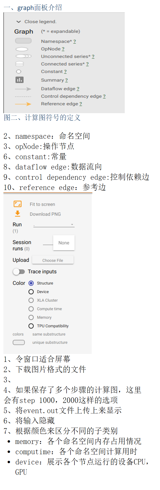
面板介绍
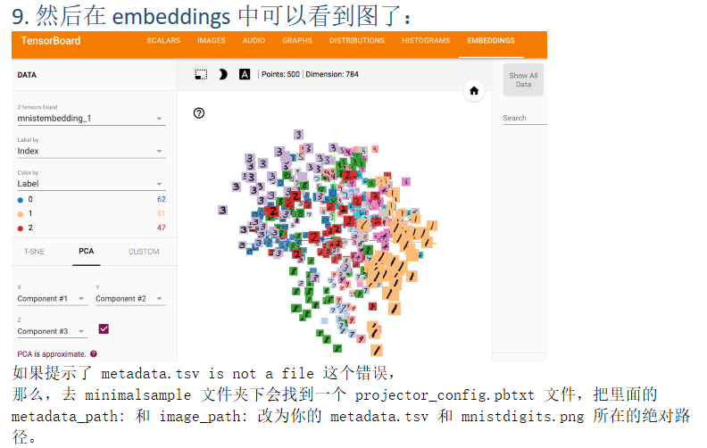
embeddings 高维可视化
来自 <https://blog.csdn.net/aliceyangxi1987/article/details/71079387>
第一步、指定一个2D的张量来储存嵌入
embedding_var = tf.Variable(…)
第二步、在LOG_DIR中保存模型
saver = tf.train.Saver()
saver.save(session,os.path.join(LOG_DIR,'model_name.ckpt),step)

1. 引入 projector,data,定义 path:
%matplotlib inline
import matplotlib.pyplot as plt
import tensorflow as tf
import numpy as np
import os

from tensorflow.contrib.tensorboard.plugins import projector
from tensorflow.examples.tutorials.mnist import input_data
LOG_DIR = 'minimalsample'#保存路径
NAME_TO_VISUALISE_VARIABLE = "mnistembedding"#需要可视化的变量
TO_EMBED_COUNT = 500
path_for_mnist_sprites =  os.path.join(LOG_DIR,'mnistdigits.png')
path_for_mnist_metadata =  os.path.join(LOG_DIR,'metadata.tsv')
mnist = input_data.read_data_sets("MNIST_data/", one_hot=False)
batch_xs, batch_ys = mnist.train.next_batch(TO_EMBED_COUNT)
2. 建立 embeddings,
也就是前面的第一步,最主要的就是你要知道想可视化查看的 variable 的名字
embedding_var = tf.Variable(batch_xs, name=NAME_TO_VISUALISE_VARIABLE)
#这一步是制定了一个变量,并给他起了一个名字
summary_writer = tf.summary.FileWriter(LOG_DIR)#创建一个writer
3. 建立 embedding projector
这一步很重要,要指定想要可视化的 variable,metadata 文件的位置
config = projector.ProjectorConfig()
embedding = config.embeddings.add()
embedding.tensor_name = embedding_var.name

# 指定metadata的位置
embedding.metadata_path = path_for_mnist_metadata #'metadata.tsv'
# 指定sprite位置 (we will create this later)
embedding.sprite.image_path = path_for_mnist_sprites #'mnistdigits.png'
embedding.sprite.single_image_dim.extend([28,28])
# Say that you want to visualise the embeddings
projector.visualize_embeddings(summary_writer, config)
4. 保存,即上面第二步:
Tensorboard 会从保存的图形中加载保存的变量,所以初始化 session 和变量,并将其保存在 logdir 中,
sess = tf.InteractiveSession()
sess.run(tf.global_variables_initializer())
saver = tf.train.Saver()
saver.save(sess, os.path.join(LOG_DIR, "model.ckpt"), 1)
5. 定义 helper functions:
**create_sprite_image:** 将 sprits 整齐地对齐在方形画布上
**vector_to_matrix_mnist:** 将 MNIST 的 vector 数据形式转化为 images
**invert_grayscale: **将黑背景变为白背景

def create_sprite_image(images):
    """Returns a sprite image consisting of images passed as argument. Images should be count x width x height"""
    if isinstance(images, list):
        images = np.array(images)
    img_h = images.shape[1]
    img_w = images.shape[2]
    n_plots = int(np.ceil(np.sqrt(images.shape[0])))


    spriteimage = np.ones((img_h * n_plots ,img_w * n_plots ))

    for i in range(n_plots):
        for j in range(n_plots):
            this_filter = i * n_plots + j
            if this_filter < images.shape[0]:
                this_img = images[this_filter]
                spriteimage[i * img_h:(i + 1) * img_h,
                  j * img_w:(j + 1) * img_w] = this_img

    return spriteimage
def vector_to_matrix_mnist(mnist_digits):
#返回的是矩阵形式
    """Reshapes normal mnist digit (batch,28*28) to matrix (batch,28,28)"""
    return np.reshape(mnist_digits,(-1,28,28))
def invert_grayscale(mnist_digits):
    """ Makes black white, and white black """
    return 1-mnist_digits
6. 保存 sprite image:
将 vector 转换为 images,反转灰度,并创建并保存 sprite image。

to_visualise = batch_xs
to_visualise = vector_to_matrix_mnist(to_visualise)
to_visualise = invert_grayscale(to_visualise)

sprite_image = create_sprite_image(to_visualise)

plt.imsave(path_for_mnist_sprites,sprite_image,cmap='gray')
plt.imshow(sprite_image,cmap='gray')
7. 保存 metadata:
将数据写入 metadata,因为如果想在可视化时看到不同数字用不同颜色表示,需要知道每个 image 的标签,在这个 metadata 文件中有这样两列:”Index” , “Label”

with open(path_for_mnist_metadata,'w') as f:
    f.write("Index	Label
")
    for index,label in enumerate(batch_ys):
        f.write("%d	%d
" % (index,label))
8. 执行:
我是用 jupyter notebook 写的,执行前面的代码后,会在当前 ipynb 所在文件夹下生成一个 minimalsample 文件夹,

要打开 tensorboard ,需要在终端执行:

$ tensorboard --logdir=YOUR FOLDER/minimalsample

---------------------
作者:Alice熹爱学习
来源:CSDN
原文:https://blog.csdn.net/aliceyangxi1987/article/details/71079387
版权声明:本文为博主原创文章,转载请附上博文链接!
tensorboard记录的种类
