Abstract—Multiobjective evolutionary algorithms (EAs) that use nondominated sorting and sharing have been criticized mainly for their:
1) O(MN3) computational complexity (where is the number of objectives and is the population size);
2) nonelitism approach; and
3) the need for specifying a sharing parameter.
In this paper, we suggest a nondominated sorting-based multiobjective EA (MOEA), called nondominated sorting genetic algorithm II (NSGA-II), which alleviates all the above three difficulties. Specifically, a fast nondominated sorting approach with O(MN2) computational complexity is presented. Also, a selection operator is presented that creates a mating pool by combining the parent and offspring populations and selecting the best (with respect to fitness and spread) solutions. Simulation results on difficult test problems show that the proposed NSGA-II, in most problems, is able to find much better spread of solutions and better convergence near the true Pareto-optimal front compared to Pareto-archived evolution strategy and strength-Pareto EA—two other elitist MOEAs that pay special attention to creating a diverse Pareto-optimal front.Moreover, we modify the definition of dominance in order to solve constrained multiobjective problems efficiently. Simulation results of the constrained NSGA-II on a number of test problems, including a five-objective seven-constraint nonlinear problem, are compared with another constrained multiobjective optimizer and much better performance of NSGA-II is observed.
概述——利用非支配排序算法多目标进化算法,有共同的缺点:
1)时间复杂度O(MN3)
2)非精英主义方法
3)明确共享参数的需求
在这篇论文中,我们提出一个非支配多目标进化算法,成为非支配排序进化算法2(NSGA-II),减轻了前三种问题。特别地,提出了一个时间复杂度为O(MN2)快速的非支配排序方法。并且, 结合亲代和子代种群创造匹配池的选择运算符,选择最优解(考虑适应度和传播)。在复杂测试问题上模拟结果,展示了提出的NSGA2,在大多数问题,是能够找到一个更好的解分布,相较于之前的其他两种更关注于创造一个多样化的Pareto optimal front的精英多目标进化——Pareto-archive进化策略和strength-Pareto进化算法,该方法在真Pareto最优前沿的附近更好收敛。此外,为了有效解决约束的多目标问题,我们修改支配的定义。约束的NSGAII的模拟解集,在包括五个目标七个约束的非线性问题一系列测试问题上得出,作为和和另一个约束的多目标优化器的比较,有更好的表现。
A. Fast Nondominated Sorting Approach
For the sake of clarity, we first describe a naive and slow procedure of sorting a population into different nondomination levels. Thereafter, we describe a fast approach.
In a naive approach, in order to identify solutions of the first nondominated front in a population of size , each solution can be compared with every other solution in the population to find if it is dominated. This requires O(MN) comparisons for each solution, where M is the number of objectives. When this process is continued to find all members of the first nondominated level in the population, the total complexity is O(MN2) .At this stage, all individuals in the first nondominated front are found. In order to find the individuals in the next nondominated front, the solutions of the first front are discounted temporarily and the above procedure is repeated.
一个快速的非支配搜索算法
为了简洁,我们先描述了一个原始慢速的种群支配等级排序过程,在此之后描述快速的方法。
在原始方法中,为了在种群大小中辨识第一支配前沿的解集,每个解与种群中的其他解做比较来发现其是否受支配。每个解需要 O(MN)次比较,M是目标数。当继续这个过程来发现所有第一支配顺位的成员,总的复杂度是O(MN2)。这个阶段,找到所有在第一支配前沿的个体。为了找到在下一个非支配前沿的个体,在第一前沿的解集暂时不被计算,重复上述过程。
In the worst case, the task of finding the second front also requires O(MN2) computations, particularly when O(N) number of solutions belong to the second and higher nondominated levels. This argument is true for finding third and higher levels of nondomination. Thus, the worst case is when there are fronts and there exists only one solution in each front. This requires an overall O(MN3) computations. Note that O(N) storage is required for this procedure. In the following paragraph and equation shown at the bottom of the page, we describe a fast nondominated sorting approach which will require O(MN2) computations.
在最坏的场合,找到第二前沿也需要O(MN2)次计算,特别当O(N)为属于第二和更高的非支配等级解的数目。为了找到第三或更高非支配等级,这个声明为真。因此最坏的情况是这有许多前沿并且每个前沿仅存在一个解。这需要整体的计算(O(MN3)次)。注意这个过程需要O(N)次存储。在下面的段落和本页底部展示的方程,我们描述了一个需要O(MN2)次计算的快速非支配排序方法。
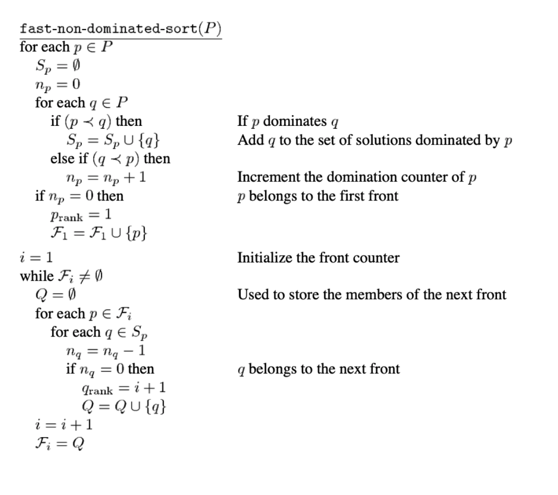
First, for each solution we calculate two entities: 1) domination count , the number of solutions which dominate the solution , and 2) , a set of solutions that the solution dominates. This requires O(MN2) comparisons.
首先,对于每个解我们计算两个实体:1)受支配数,支配当前解的其他解的数目,2)当前解所支配的一系列解集。这需要O(MN2)次比较。
All solutions in the first nondominated front will have their domination count as zero. Now, for each solution p with np = 0 , we visit each member (q) of its set Sp and reduce its domination count by one. In doing so, if for any member q the domination count becomes zero, we put it in a separate list Q. These members belong to the second nondominated front. Now, the above procedure is continued with each member of Q and the third front is identified. This process continues until all fronts are identified.
所有在第一支配前沿的解的受支配数为零。现在,对于每个np = 0的解p,我们遍历对应集合Sp的每个成员(q),使其受支配数减一。在这么做的过程中,如果任意成员的受支配数变为0,我们将它放入另一个列表Q里。这些成员属于第二非支配前沿。现在,Q的成员继续上述过程,并且找到第三前沿。这个过程继续直到找到所有前沿。
For each solution p in the second or higher level of nondomination, the domination count np can be at most N-1. Thus, each solution p will be visited at most N-1 times before its domination count becomes zero. At this point, the solution is assigned a nondomination level and will never be visited again.Since there are at most N-1 such solutions, the total complexity is O(N2). Thus, the overall complexity of the procedure is O(MN2). Another way to calculate this complexity is to realize that the body of the first inner loop (for each p ∈ Fi) is executed exactly N times as each individual can be the member of at most one front and the second inner loop (for each q ∈ Sq ) can be executed at maximum (N-1) times for each individual [each individual dominates(N -1) individuals at maximum and each domination check requires at most M comparisons] results in the overall O(MN2) computations. It is important to note that although the time complexity has reduced to O(MN2), the storage requirement has increased to O(N2).
对于每个在第二或更高的非支配层的解p,受支配数np最大为N-1。因此在其受支配数变为零之前,每个解p最多会被遍历N-1次。出于这点,解被分配一个非支配等级并且将不会被再次访问。因此有最多N-1个这样的解,整体的复杂度为O(N2)。因此该流程整体的复杂度为O(MN2)。另一个计算复杂度的方法是实现第一次内部循环体(for each p ∈ Fi),恰好运行N次因为每个个体最多属于一个前沿。对于每个个体而言,第二前沿的内部循环(for each q ∈ Sq )最多运行N-1次[每个个体最多主导N-1个个体,每个支配查询需要最多M次比较],因此总共需要O(MN2)次计算。值得一提的是,虽然时间复杂度减少到O(MN2),但是存储需求增长到了O(N2)。
上图中的比较符号可为离散数学中的偏序关系
B. Diversity Preservation
We mentioned earlier that, along with convergence to the Pareto-optimal set, it is also desired that an EA maintains a good spread of solutions in the obtained set of solutions. The original NSGA used the well-known sharing function approach, which has been found to maintain sustainable diversity in a population with appropriate setting of its associated parameters. The sharing function method involves a sharing parameter σshare, which sets the extent of sharing desired in a problem. This parameter is related to the distance metric chosen to calculate the proximity measure between two population members. The parameter denotes the largest value of that distance metric within which any two solutions share each other’s fitness. This parameter is usually set by the user, although there exist some guidelines [4]. There are two difficulties with this sharing function approach.
1) The performance of the sharing function method in maintaining a spread of solutions depends largely on the chose σshare value.2) Since each solution must be compared with all other solutions in the population, the overall complexity of the sharing function approach is O(N2)
我们之前提到,在收敛到Pareto最优集是,也希望进化算法在获得解集上维持一个好的分布。原生的NSGA使用有名的的共享函数功能,共享函数配置合适的相关参数,可维持种群的持续多样性。共享函数方法涉及到共享参数 σshare,其设置了问题中共享的范围。这个参数和计算两个种群成员的临近距离的米制选择有关。参数表示米制距离的最大值,在这个范围中任意两个解都共享对方的适应度。这个参数通常由用户设置,尽管有一些方针指示。共享函数方法有两个难题:
1)共享函数在维持解分布上的表现在很大程度上依赖于σshare的选择
2)由于每个解需要和其他在种群中的解比较,共享函数法的总体复杂度为O(N2)
In the proposed NSGA-II, we replace the sharing function approach with a crowded-comparison approach that eliminates both the above difficulties to some extent. The new approach does not require any user-defined parameter for maintaining diversity among population members. Also, the suggested approach has a better computational complexity. To describe this approach, we first define a density-estimation metric and then present the crowded-comparison operator.
在提出的NSGA-II算法中,我们用拥挤度比较方法取代共享函数方法,限制上述两种拓展困难。这个新方法不需要任何用户定义参数来维持种群成员的多样性。且有更好的计算复杂度。为了描述这个方法,我们先定义一个密度评估米制,然后表示密度比较算子。
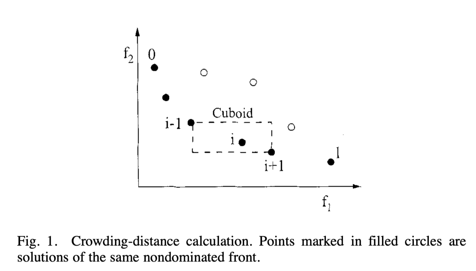
1) Density Estimation: To get an estimate of the density of solutions surrounding a particular solution in the population, we calculate the average distance of two points on either side of this point along each of the objectives. This quantity idistance serves as an estimate of the perimeter of the cuboid formed by using the nearest neighbors as the vertices (call this the crowding distance). In Fig. 1, the crowding distance of the ith solution in its front (marked with solid circles) is the average side length of the cuboid (shown with a dashed box).
1)密度评估:为了估计在种群中特定解附近的解集密度,我们沿着对应目标计算这个解两侧的两点间的距离均值。这个距离值idistance被用作以最近相邻作为顶点数的立方体的边缘检测(称为拥挤距离)。在图1中,在解i前沿的拥挤距离(用实心圆表示)是立方体(用虚线框表示)的平均边长。
The crowding-distance computation requires sorting the population according to each objective function value in ascending order of magnitude. Thereafter, for each objective function, the boundary solutions (solutions with smallest and largest function values) are assigned an infinite distance value. All other intermediate solutions are assigned a distance value equal to the absolute normalized difference in the function values of two adjacent solutions. This calculation is continued with other objective functions. The overall crowding-distance value is calculated as the sum of individual distance values corresponding to each objective. Each objective function is normalized before calculating the crowding distance. The algorithm as shown at the bottom of the page outlines the crowding-distance computation procedure of all solutions in an nondominated set L.
拥挤距离的计算需要根据目标函数值对种群进行升序排序。因此,对于每个目标函数,边界解(对应函数最大最小值的解)分配了一个无限距离值。其他所有内部解分配了一个,与两个临近解的函数值的规范化差的绝对值相同的距离值。对于其他目标函数,继续该计算。全局的拥挤距离是,与各目标一致的每个个体的距离的加和。在计算拥挤距离前正则化每个目标函数。算法在本页底部展示了在非支配集L所有解的拥挤距离的计算流程。
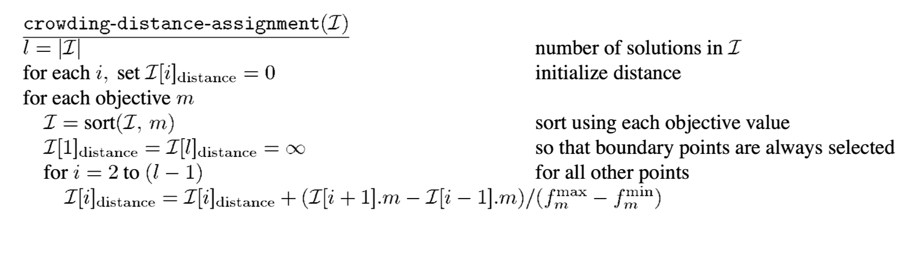
Here, L[i].m refers to the th objective function value of the ith individual in the set and the parameters and are the maximum and minimum values of the th objective function. The complexity of this procedure is governed by the sorting algorithm. Since independent sortings of at most solutions (when all population members are in one front ) are involved, the above algorithm has O(MNlogN) computational complexity.
这里的L[i].m是指集合中第i个个体的目标函数的值,参数均为目标函数的最大最小值。排序决定这个过程的复杂度。因为涉及了对最多解集(当所有种群成员都在同一前沿)的独立排序,上述算法有O(MNlogN)的计算复杂度。
After all population members in the set L are assigned a distance metric, we can compare two solutions for their extent of proximity with other solutions. A solution with a smaller value of this distance measure is, in some sense, more crowded by other solutions. This is exactly what we compare in the proposed crowded-comparison operator, described below.
Although Fig. 1 illustrates the crowding-distance computation for two objectives, the procedure is applicable to more than two objectives as well.
在集合L中所有种群成员都被分配一个米制距离,我们可以比较两个解和其他解的边缘扩展。一个具有更小距离的解,在某些场合,与其他解更拥挤。下面描述的,就是我们提出的拥挤度比较算子所比较的。虽然图1 展示了两个目标的拥挤距离的计算,这个过程也可应用到大于两个目标上。
2) Crowded-Comparison Operator: The crowded-comparison operator ( ≺n ) guides the selection process at the various stages of the algorithm toward a uniformly spread-out Pareto- optimal front. Assume that every individual in the population has two attributes:
1) nondomination rank ( irank );
2) crowding distance ( idistance ).
We now define a partial order ≺n asi ≺n j if ( irank < jrank )
or (( irank = jrank)
and ( idistance > jdistance))
That is, between two solutions with differing nondomination ranks, we prefer the solution with the lower (better) rank. Otherwise, if both solutions belong to the same front, then we prefer the solution that is located in a lesser crowded region.
With these three new innovations—a fast nondominated sorting procedure, a fast crowded distance estimation procedure, and a simple crowded comparison operator, we are now ready to describe the NSGA-II algorithm.
拥挤比较算子:拥挤比较算子≺n指导不同的算法阶段中选择的过程向着均匀分布的Pareto最优前沿前进。假设每个在种群中的解有两个属性
1)非支配排行irank
2)拥挤距离idistance
我们现在定义偏序符号≺n:
i ≺n j if ( irank < jrank )
or (( irank = jrank)
and ( idistance > jdistance))
也就是说,在两个有不同的非支配排行的解之间,我们选择具有更低(更好)排行的解。否则,如果两个解都属于同一前沿,我们选择在更稀疏拥挤区域的解。
结合这三个新的创新,一个快速非支配排行过程,一个快速的拥挤距离估计过程,和一个简单的拥挤度比较算子,我们可以描述NSGA-II算法了。
C. Main Loop
Initially, a random parent population is created. The population P0 is sorted based on the nondomination. Each solution is assigned a fitness (or rank) equal to its nondomination level (1 is the best level, 2 is the next-best level, and so on). Thus, minimization of fitness is assumed. At first, the usual binary tournament selection, recombination, and mutation operators are used to create a offspring population Q0 of size N . Since elitism is introduced by comparing current population with previously found best nondominated solutions, the procedure is different after the initial generation. We first describe the tth generation of the proposed algorithm as shown at the bottom of the page.
C.主循环
最初,创建一个随机的亲代种群。非支配排序种群P0。每个解都分配一个与其非支配等级相等的适应度(或者排行)(一级是最好的,二级次之,以此类推)。因此,假设一个最小的适应度。首先,常见的二分比较选择,重构,和变异运算符被用来创建种群大小为N的子代Q0。通过比较目前种群与之前找到的最优非支配解介绍了精英主义,流程在初代种群后变得不同。在底部图片中,我们首先描述了提出算法的t代。
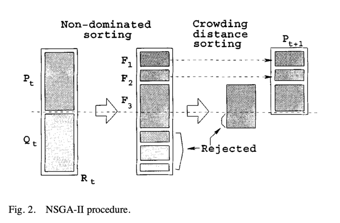
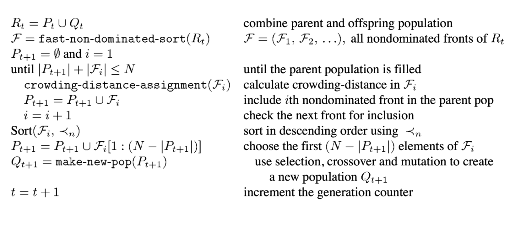
The step-by-step procedure shows that NSGA-II algorithm is simple and straightforward. First, a combined population Rt = Pt υ Qt is formed. The population Rt is of size 2N. Then, the population Rt is sorted according to nondomination. Since all previous and current population members are included in Rt, elitism is ensured. Now, solutions belonging to the best nondominated set F1 are of best solutions in the combined population and must be emphasized more than any other solution in the combined population.
一步一步地展示NSGA-II算法是简单且直接的。首先,合成种群Rt = Pt υ Qt。种群Rt的大小为2N。接下来, 对种群Rt进行非支配排序。既然Rt包含了所有之前和现在的种群成员,就保证了精英主义。现在,属于最佳的非支配集 F1的解是在合成种群中的最优解,且必须被比其他在合成种群中的解更为强调。
If the size of F1 is smaller than N, we definitely choose all members of the set F1 for the new population Pt+1. The remaining members of the population Pt+1 are chosen from subsequent nondominated fronts in the order of their ranking. Thus, solutions from the set F2 are chosen next, followed by solutions from the set F3, and so on. This procedure is continued until no more sets can be accommodated. Say that the set Fl is the last nondominated set beyond which no other set can be accommodated.
如果第一前沿F1的大小小于N,我们选择其所有成员构成新的种群Pt+1。种群Pt+1剩下的成员会从接下来的非支配前沿按照其排行选择。因此,下一步选择集合F2的解,然后是F3,并以此类推。这个过程继续指导容不下任何集合。称集合Fl为最后非支配集,在其之后没有其他的集合被加入(种群Pt+1)。
In general, the count of solutions in all sets from F1 to Fl would be larger than the population size.
To choose exactly N population members, we sort the solutions of the last front Fl using the crowded-comparison operator ≺n in descending order and choose the best solutions needed to fill all population slots.
总的来说, F1 到 Fl所有解的数目 会比种群大小更大。
为了选择正好数目为种群数N的成员,我们用拥挤度比较算子≺n对最后前沿Fl进行降序排序,并选择要填充所有种群的最优解。
The NSGA-II procedure is also shown in Fig. 2. The new population Pt+1 of size N is now used for selection, crossover, and mutation to create a new population Qt+1 of size N . It is important to note that we use a binary tournament selection operator but the selection criterion is now based on the crowded-comparison operator ≺n. Since this operator requires both the rank and crowded distance of each solution in the population Pt+1, we calculate these quantities while forming the population , as shown in the above algorithm.
图2展示了NSGA-II过程。大小为N的新种群Pt+1被用来进行选择,交叉和变异来生成新的大小为N的种群Qt+1。注意我们用二分比较选择符,这很关键,但是现在的选择标准是基于拥挤度算子≺n的选择符。因为该运算符需要在种群Pt+1中的每一个解的(非支配)排行和拥挤距离,在种群构成时,我们计算这些量,如以上算法所示。