学算法——gradient descent

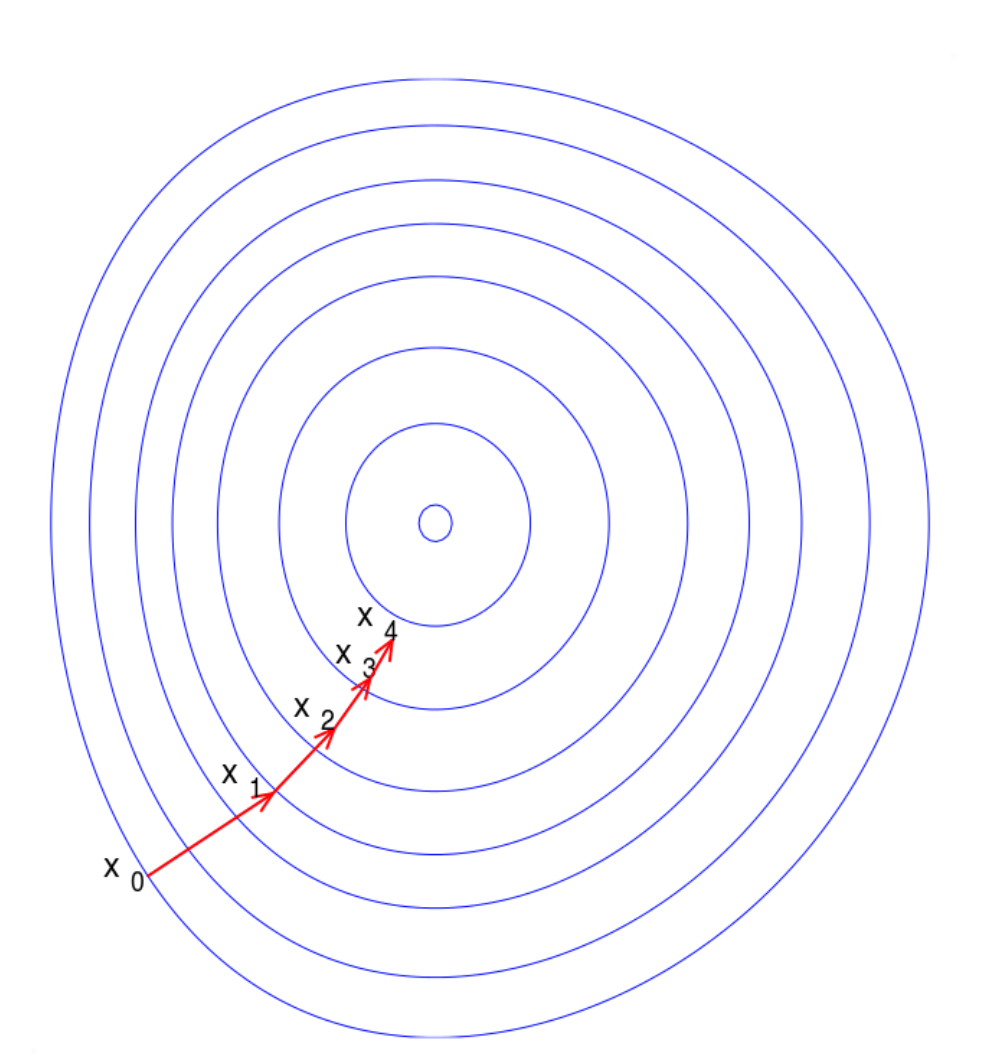
Gradient descent is a first-order iterative optimization algorithm for finding a local minimum of a differentiable function. To find a local minimum of a function using gradient descent, we take steps proportional to the negative of the gradient (or approximate gradient) of the function at the current point. But if we instead take steps proportional to the positive of the gradient, we approach a local maximum of that function; the procedure is then known as gradient ascent. Gradient descent is generally attributed to Cauchy, who first suggested it in 1847,^[1] but its convergence properties for non-linear optimization problems were first studied by Haskell Curry in 1944.^[2]

梯度下降是寻找可微函数的局部最小值的先序迭代优化算法。为了找到一个局部最小值，我们采用步长来成比例地从当前点沿着函数的负梯度或负梯度的大致方向（来接近最小值）。但是如果我们如果采用正梯度，我们会找到函数的局部最大值；这个过程称为梯度下降。总的来说，梯度下降是高斯在1847年最早提出的，但Haskell Curry在1944年最早研究了它的非线性优化问题的收敛特性。

Gradient descent is based on the observation that if the multi-variable function $F(mathbf {x} )$ is defined and differentiable in a neighborhood of a point $mathbf {a}$ , then $F(mathbf {x} )$ decreases fastest if one goes from $mathbf {a}$ in the direction of the negative gradient of $F$ at ${displaystyle mathbf {a} ,- abla F(mathbf {a} )}$ .

　　梯度下降给予对于多变量函数F(x)的观察，F(x)是定义在点a临域可导的函数，F(x)从a出发沿着a的负梯度方向 ${displaystyle mathbf {a} ,- abla F(mathbf {a} )}$ 下降地最快。

It follows that, if ${displaystyle mathbf {a} _{n+1}=mathbf {a} _{n}-gamma abla F(mathbf {a} _{n})}$ for ${displaystyle gamma in mathbb {R} _{+}}$ small enough, then ${displaystyle F(mathbf {a_{n}} )geq F(mathbf {a_{n+1}} )}$ .

每次迭代 ${displaystyle mathbf {a} _{n+1}=mathbf {a} _{n}-gamma abla F(mathbf {a} _{n})}$ ， ${displaystyle gamma in mathbb {R} _{+}}$ 是很小的步长，可得到 ${displaystyle F(mathbf {a_{n}} )geq F(mathbf {a_{n+1}} )}$

In other words, the term ${displaystyle gamma abla F(mathbf {a} )}$ is subtracted from $mathbf {a}$ because we want to move against the gradient, toward the local minimum. With this observation in mind, one starts with a guess $mathbf {x} _{0}$ for a local minimum of $F$ , and considers the sequence ${displaystyle mathbf {x} _{0},mathbf {x} _{1},mathbf {x} _{2},ldots }$ such that $mathbf {x} _{n+1}=mathbf {x} _{n}-gamma _{n} abla F(mathbf {x} _{n}), ngeq 0.$

换种说法，从a点（处的值）减去 ${displaystyle gamma abla F(mathbf {a} )}$ ，因为我们想逆着梯度，向着局部最小值移动。记住这个观察量，从一个猜测点 $mathbf {x} _{0}$ 开始向着函数 $F$ 的局部最小移动，考虑序列 ${displaystyle mathbf {x} _{0},mathbf {x} _{1},mathbf {x} _{2},ldots }$ 可以得到 $mathbf {x} _{n+1}=mathbf {x} _{n}-gamma _{n} abla F(mathbf {x} _{n}), ngeq 0.$

We have a monotonic sequence

$F(mathbf {x} _{0})geq F(mathbf {x} _{1})geq F(mathbf {x} _{2})geq cdots ,$

so hopefully the sequence $(mathbf {x} _{n})$ converges to the desired local minimum. Note that the value of the step size $gamma$ is allowed to change at every iteration. With certain assumptions on the function $F$ (for example, $F$ convex and $abla F$ Lipschitz) and particular choices of $gamma$ (e.g., chosen either via a line search that satisfies the Wolfe conditions, or the Barzilai–Borwein method^[3]^[4] shown as following),

${displaystyle gamma _{n}={frac {left|left(mathbf {x} _{n}-mathbf {x} _{n-1} ight)^{T}left[ abla F(mathbf {x} _{n})- abla F(mathbf {x} _{n-1}) ight] ight|}{left| abla F(mathbf {x} _{n})- abla F(mathbf {x} _{n-1}) ight|^{2}}}}$

我们获得了单调序列， $F(mathbf {x} _{0})geq F(mathbf {x} _{1})geq F(mathbf {x} _{2})geq cdots ,$ 希望序列 $(mathbf {x} _{n})$ 收敛于期望的局部最小。记录步长 $gamma$ 的值每次迭代可变。在对函数 $F$ 的确定假设下（例如凸函数 $F$ 和函数的导数 Lipschitz函数 $abla F$ ），和指定的 $gamma$ 值选择（例如，通过线性搜索选择一个 $gamma$ 满足Wolfe conditions*或 Barzilai–Borwein*方法）...

convergence to a local minimum can be guaranteed. When the function $F$ is convex, all local minima are also global minima, so in this case gradient descent can converge to the global solution.

$gamma$ 收敛于一个可保证的局部最小，当函数F为凸函数是，所有局部最小均为全局最小，所以在这种情况，梯度下降可收敛于全局解。

Solution of a linear system

Gradient descent can be used to solve a system of linear equations, reformulated as a quadratic minimization problem, e.g., using linear least squares. The solution of

$Amathbf {x} -mathbf {b} =0$

in the sense of linear least squares is defined as minimizing the function ${displaystyle F(mathbf {x} )=left|Amathbf {x} -mathbf {b} ight|^{2}.}$

线性空间的解

梯度下降可以解线性方程组，用线性最小二乘重新定义求二次曲线最小值的问题。 $Amathbf {x} -mathbf {b} =0$ 的解在线性最小二乘可定义为最小化函数 ${displaystyle F(mathbf {x} )=left|Amathbf {x} -mathbf {b} ight|^{2}.}$

In traditional linear least squares for real $A$ and $mathbf {b}$ the Euclidean norm is used, in which case $abla F(mathbf {x} )=2A^{T}(Amathbf {x} -mathbf {b} ).$

In this case, the line search minimization, finding the locally optimal step size $gamma$ on every iteration, can be performed analytically, and explicit formulas for the locally optimal $gamma$ are known.^[6]

在传统的线性最小二乘中，对于实值的向量矩阵A和b使用了欧几里得范数，如在对向量矩阵构成的函数求导的场合 $abla F(mathbf {x} )=2A^{T}(Amathbf {x} -mathbf {b} ).$ 在线性搜索最小值的情况，每一次迭代可分析得到一个局部最优步长 $gamma$ ，并精确组成局部已知最优 $gamma$ 集。

The algorithm is rarely used for solving linear equations, with the conjugate gradient method being one of the most popular alternatives. The number of gradient descent iterations is commonly proportional to the spectral condition number $kappa (A)$ of the system matrix $A$ (the ratio of the maximum to minimum eigenvalues of $A^{T}A$ ), while the convergence of conjugate gradient method is typically determined by a square root of the condition number, i.e., is much faster. Both methods can benefit from preconditioning, where gradient descent may require less assumptions on the preconditioner.^[7]

算法很少用来解决线性方程，因为共轭梯度算法*是一个很火的选项。梯度下降的迭代数是与系统矩阵A成比例的光谱条件数 $kappa (A)$ 所共有的（ $A^{T}A$ 最大到最小的（分割）比率）。一个典型的情况：当条件数的平方根决定共轭梯度法收的收敛时，这种方法比梯度下降收敛更快。两种方法都受益于预条件，其中梯度下降需要对预条件子更少的假设。

Solution of a non-linear system

Gradient descent can also be used to solve a system of nonlinear equations. Below is an example that shows how to use the gradient descent to solve for three unknown variables, x₁, x₂, and x₃. This example shows one iteration of the gradient descent.

梯度下降也用来解决非线性问题。这里有一个相关的例子，用梯度下降法求解三个未知数 x₁, x₂, 和x₃_。这个例子展示了梯度下降的一次迭代。

Consider the nonlinear system of equations

${displaystyle {egin{cases}3x_{1}-cos(x_{2}x_{3})-{ frac {3}{2}}=0\4x_{1}^{2}-625x_{2}^{2}+2x_{2}-1=0\exp(-x_{1}x_{2})+20x_{3}+{ frac {10pi -3}{3}}=0end{cases}}}$

Let us introduce the associated function

${displaystyle G(mathbf {x} )={egin{bmatrix}3x_{1}-cos(x_{2}x_{3})-{ frac {3}{2}}\4x_{1}^{2}-625x_{2}^{2}+2x_{2}-1\exp(-x_{1}x_{2})+20x_{3}+{ frac {10pi -3}{3}}\end{bmatrix}},}$

where

${displaystyle mathbf {x} ={egin{bmatrix}x_{1}\x_{2}\x_{3}\end{bmatrix}}.}$

One might now define the objective function

${displaystyle F(mathbf {x} )={frac {1}{2}}G^{mathrm {T} }(mathbf {x} )G(mathbf {x} )={frac {1}{2}}left[left(3x_{1}-cos(x_{2}x_{3})-{frac {3}{2}} ight)^{2}+left(4x_{1}^{2}-625x_{2}^{2}+2x_{2}-1 ight)^{2}+left(exp(-x_{1}x_{2})+20x_{3}+{frac {10pi -3}{3}} ight)^{2} ight],}$

which we will attempt to minimize.

_{F(x)是我们要进行梯度下降求最小值的方程}

As an initial guess, let us use

${displaystyle mathbf {x} ^{(0)}=mathbf {0} ={egin{bmatrix}0\0\0\end{bmatrix}}.}$

We know that

${displaystyle mathbf {x} ^{(1)}=mathbf {0} -gamma _{0} abla F(mathbf {0} )=mathbf {0} -gamma _{0}J_{G}(mathbf {0} )^{mathrm {T} }G(mathbf {0} ),}$

where the Jacobian matrix ${displaystyle J_{G}}$ is given by ${displaystyle J_{G}(mathbf {x} )={egin{bmatrix}3&sin(x_{2}x_{3})x_{3}&sin(x_{2}x_{3})x_{2}\8x_{1}&-1250x_{2}+2&0\-x_{2}exp {(-x_{1}x_{2})}&-x_{1}exp(-x_{1}x_{2})&20\end{bmatrix}}.}$

初始猜测x^₍₀₎为3*1的零矩阵，通过递归下降的迭代转移公式，推导得到x⁽¹⁾,其中J_G(x)为矩阵G(x)对x求导所得。（由前文可得，gama由经验值设定）

We calculate:

${displaystyle J_{G}(mathbf {0} )={egin{bmatrix}3&0&0\0&2&0\0&0&20end{bmatrix}},qquad G(mathbf {0} )={egin{bmatrix}-2.5\-1\10.472end{bmatrix}}.}$ Thus ${displaystyle mathbf {x} ^{(1)}=mathbf {0} -gamma _{0}{egin{bmatrix}-7.5\-2\209.44end{bmatrix}},}$

and ${displaystyle F(mathbf {0} )=0.5left((-2.5)^{2}+(-1)^{2}+(10.472)^{2} ight)=58.456.}$ Now, a suitable $gamma _{0}$ must be found such that ${displaystyle Fleft(mathbf {x} ^{(1)} ight)leq Fleft(mathbf {x} ^{(0)} ight)=F(mathbf {0} ).}$

This can be done with any of a variety of line search algorithms. One might also simply guess ${displaystyle gamma _{0}=0.001,}$ which gives ${displaystyle mathbf {x} ^{(1)}={egin{bmatrix}0.0075\0.002\-0.20944\end{bmatrix}}.}$

Evaluating the objective function at this value, yields ${displaystyle Fleft(mathbf {x} ^{(1)} ight)=0.5left((-2.48)^{2}+(-1.00)^{2}+(6.28)^{2} ight)=23.306.}$

The decrease from ${displaystyle F(mathbf {0} )=58.456}$ to the next step's value of ${displaystyle Fleft(mathbf {x} ^{(1)} ight)=23.306}$

第一次迭代不同gama值的详细过程