Python之密度聚类

 1 # -*- coding: utf-8 -*-
 2 """
 3 Created on Tue Sep 25 10:48:34 2018
 4 
 5 @author: zhen
 6 """
 7 
 8 import numpy as np
 9 import matplotlib.pyplot as plt
10 import sklearn.datasets as ds
11 import matplotlib.colors
12 from sklearn.cluster import DBSCAN
13 from sklearn.preprocessing import StandardScaler
14 
15 def expand(a, b):
16     d = (b - a) * 0.1
17     return a-d, b+d
18 
19 if __name__ == "__main__":
20     N = 1000
21     centers = [[1, 2], [-1, -1], [1, -1], [-1, 1]]
22     data, y = ds.make_blobs(N, n_features=2, centers=centers, cluster_std=[0.5, 0.25, 0.7, 0.5], random_state=0)
23     # 归一化数据
24     data = StandardScaler().fit_transform(data)
25     # 数据的参数
26     params = ((0.2, 5), (0.2, 10), (0.2, 15), (0.3, 5), (0.3, 10), (0.3, 15))
27     
28     # 设置中文样式
29     matplotlib.rcParams['font.sans-serif'] = [u'SimHei']
30     matplotlib.rcParams['axes.unicode_minus'] = False
31     # 设置颜色
32     cm = matplotlib.colors.ListedColormap(list('rgbm'))
33     plt.figure(figsize=(12, 8), facecolor='w')
34     plt.suptitle(u'DBSCAN聚类', fontsize=20)
35     
36     for i in range(6):
37         eps, min_samples = params[i]
38         # 创建密度聚类模型
39         model = DBSCAN(eps=eps, min_samples=min_samples)
40         # 训练模型
41         model.fit(data)
42         y_hat = model.labels_
43         
44         core_indices = np.zeros_like(y_hat, dtype=bool)
45         core_indices[model.core_sample_indices_] = True
46         
47         y_unique = np.unique(y_hat)
48         n_clusters = y_unique.size - (1 if -1 in y_hat else 0)
49         # print(y_unique, '聚类簇的个数：', n_clusters)
50         
51         plt.subplot(2, 3, i+1)
52         clrs = plt.cm.Spectral(np.linspace(0, 0.8, y_unique.size))
53         # print(clrs)
54         
55         x1_min, x2_min = np.min(data, axis=0)
56         x1_max, x2_max = np.max(data, axis=0)
57         x1_min, x1_max = expand(x1_min, x1_max)
58         x2_min, x2_max = expand(x2_min, x2_max)
59         
60         for k, clr in zip(y_unique, clrs):
61             cur = (y_hat == k)
62             if k == -1:
63                 plt.scatter(data[cur, 0], data[cur, 1], s=20, c='k')
64             # 设置散点图数据
65             plt.scatter(data[cur, 0], data[cur, 1], s=20, cmap=cm, edgecolors='k')
66             plt.scatter(data[cur & core_indices][:, 0], data[cur & core_indices][:, 1], 
67                         s=20, cmap=cm, marker='o', edgecolors='k')
68         # 设置x,y轴
69         plt.xlim((x1_min, x1_max))
70         plt.ylim((x2_min, x2_max))
71         plt.grid(True)
72         plt.title(u'epsilon = %.1f m = %d, 聚类数目：%d' % (eps, min_samples, n_clusters), fontsize=16)
73     plt.tight_layout()
74     plt.subplots_adjust(top=0.9)
75     plt.show()
76

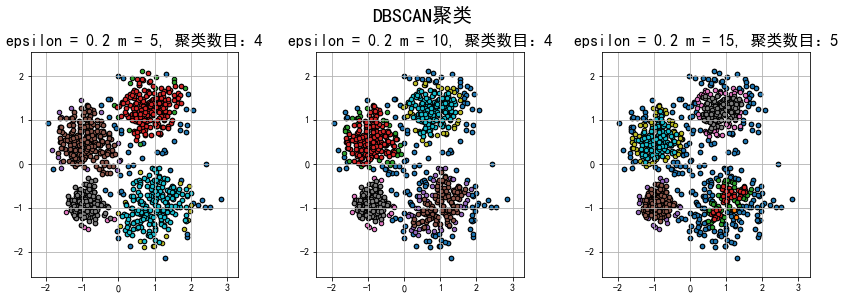
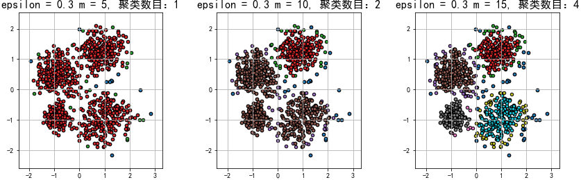
结果：

总结：

　　1.在epsilon（半径）相同的情况下，m（数量）越大，划分的聚类数目就可能越多，异常的数据就会划分的越多。在m（数量）相同的情况下，epsilon（半径）越大，划分的聚类数目就可能越少，异常的数据就会划分的越少。因此，epsilon和m是相互牵制的，合适的epsilon和m有利于更好的聚类，减少欠拟合或过拟合的情况。

　　2.和KMeans聚类相比，DBSCAN密度聚类更擅长聚不规则形状的数据，因此在数据不是接近圆形的方式分布的情况下，建议使用密度聚类！