Local Overlap Measures (Relationship between u and v) : \(S[u,v]=\frac{|\mathcal N(u)\bigcap\mathcal N(v)|}{|\mathcal N(u)\bigcup\mathcal N(v)|}\)
expected edges between nodes(rewired network)
\(E[A[u,v]]=\frac{d_ud_v}{2m};E(G)=\frac 1 2\sum_{i\in N}\sum_{j\in N}\frac{k_ik_j}{2m}= m\)
Graph modularity: \(Q=\frac 1 {2m}\sum_{s\in S}\sum_{i\in s}\sum_{j\in s}(A_{ij}-\frac {k_ik_j}{2m})\) , which is normalized to be \(-1\le Q\le 1\)
对于不相交的 clustering , 最小化 modularity:Louvain Algorithm (一种贪心算法):
Phase 1: 每个点计算如果加入邻居所在的 cluster 后的 \(\Delta Q=\frac 1 {2m}\big [\sum k_{i,in}-\frac{(\sum_{tot}+k_i)^2-(\sum_{tot})^2-k_i^2}{2m}\big ]\) ,如果最大的>0选择加入。
Phase 2: Aggregation. 然后迭代进行 Phase 1.
Leicht similarity: \(\frac {A^i}{\mathbb E[A^i]}\) (i steps)
Random Walk Matrix (for probability) :\(D^{-1}A\)
Clustering coefficient(for undirected graph)
Node i with degree ki: \(C_i=\frac{2e_i}{k_i(k_i-1)},C\in[0,1],e_i\) is the number of edges between the neighbors of node i.
Average.clustering: \(C=\frac 1 N\sum_{i=1}^N C_i\)
For erdos-renyi graph: expected E[e_i] is: \(p\frac{k_i(k_1-1)}{2}\) and E[C_i]= \(\frac{2e_i}{k_i(k_i-1)}=p=\frac{\bar k}{n-1}(ps.\bar k=p(n-1))\)
erdos-renyi graph's average path length: O(log n)
erdos-renyi graph's largest connected component: when \(\bar k>1\) ,it tends to be the whole graph.
Connectivity: how many components, the number of nodes in the largest component.
Graphlet Degree Vector(GDV): a vector with the frequency of the node in each orbit position.(graphlets on 2 to 5 nodes, vector of 73 coordinates).
Graph Isomorphism
Graphs G and H are isomorphic if there exists a bijection f: \(V(G)\rightarrow V(H)\) , such that \(\forall u,v\in G\) such that \((u,v)\in \mathcal E(G)\) ,satisfy \((f(u),f(v))\in \mathcal E(H)\)
Graph Cut: \(cut(A,B)=\sum_{i\in A,j\in B} w_{ij}\)
\(\phi(A,B)=\frac{cut(A,B)}{min(vol(A),vol(B))}\)
Graph Volume: \(vol(A)=\sum_{u\in A}d_u\)
Graph Laplacian Matrix
定义为 \(L = D - A\)
满足性质:
-
\(L\) 半正定
proof.
\(\begin{aligned}\forall x\in \R^n,x^TLx&=\sum\limits_{i=1}^nd_ix_i^2-\sum\limits_{i,j=1}^na_{ij}x_ix_j\\&=\sum\limits_{i=1}^n\sum\limits_{j=1}^na_{ij}x_i^2-\sum\limits_{i,j=1}^n a_{ij}x_ix_j\\&=\frac 1 2\Big(\sum\limits_{i,j=1}^na_{ij}x_i^2-2\sum\limits_{i,j=1}^n a_{ij}x_ix_j-\sum_{i,j=1}^na_{ij}x_j^2\Big)\\&=\frac 1 2\sum_{i,j=1}^na_{ij}(x_i-x_j)^2\ge 0\end{aligned}\)
另外有 \(x^TLx=\sum\limits_{(u,v)\in\mathcal E}(x_u-x_v)^2\)
-
\(L\) 必有 0 特征值
proof. \(L\) 每一行之和为 0,故 \((1,1,\cdots ,1)^T\) 作为 0 的特征向量。
-
\(L\) 的 0 的几何重数与连通分量个数相同
proof. 考虑到特征向量 \(v_0\) 满足 \(v_0^TLv_0=\sum\limits_{(u,v)\in\mathcal E}(x_u-x_v)^2=0\) ,所以每个连通分量取值相同。
所以 0 的特征向量张成的空间可以被形如 \((1,0,\cdots,1,0,\cdots)^T,(0,1,0,\cdots)^T\) 的向量所张成。那么几何重数就显而易见了。
-
\(L\) 可以写成 \(N^TN\) 的形式(由1得)
-
对于第二小的特征值 \(\lambda_2=\min_{x:x^Tw_1=0}\frac{x^TLx}{x^Tx}\)
由于对应的 \(w_1=(1,1,\cdots,1)^T\) , 所以 \(x^Tw_1=0\Leftrightarrow \sum_i x_i=0\)
所以有 \(\lambda_2=\min_{\sum_ix_i=0}\frac{\sum _{(u,v)\in \mathcal E}(x_u-x_v)^2}{\sum_ix_i^2}\)
对于一个二分图最小割 (二分类) 问题,可以考虑利用 \(\lambda_2\) 对应的 \(w_2\) 的分量符号作为划分依据(Rayeigh Theorem):
定义 "conductance" of the cut (A,B) is \(\beta=\frac{\#edges\ from\ A\ to\ B}{|A|}\)
1)对于最优解,记 \(|A|\le|B|,a=|A|,b=|B|\) 。现在定义:
2)有:
Motif Conductance
Motif Volume: \(vol_M(S)=\#motif\ end-points\ in\ S\)
Motif Conductance: \(\phi(S)=\frac{\#motifs\ cut}{vol_M(S)}\)
Optimizing Motif Conductance
(1) Pre-processing: Construct \(W_{ij}^{(M)}=\#times\ edge\ (i,j)\ participates\ int\ the\ motif\ M\)
(2) Sort nodes by the values in x: x1, x2, x3 \(\cdots\) and choose the best point (one cut to separate into two cluster) such that possesses the smallest motif conductance
(3) Apply spectral clustering to W, and \(L^{(M)}x=\lambda_2x\) ,x is the Fiedler vector
there is theory that shows \(\phi_M(S)\le 4\sqrt{\phi_M^*}\) (provably near optimal)
(For biological purposes).
Node Classification
Relational Classifiers(Do not use network info)
Markov Assumption: the label Yi of one node i depends on the labels of its neighbors Ni
Assuming there are k types of labels;
For labeled nodes, \(P(Y_k|i)=1,P(Y_{j\ne k}|i)=0\) ;
For unlabeled node, \(P(Y_j|i)=\frac 1 k\)
updating the nodes in random order: \(P(Y_k|i)=\frac 1 {|N_i|} \sum\limits_{(i,j)\in \mathcal E}W(i,j)P(Y_k|j)\)
iteratively do the job until the probability of all nodes converges or reaching the number of the iteration threshold.
Iterative classification
Belief Propagating Using Message Passing
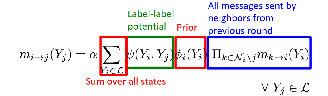
after convergence:
\(b_i(Y_i)=\) i's belief of being in state \(Y_i\)
\(b_i(Y_i)=\alpha \phi_i(Y_i)\prod_{j\in\mathcal N_i}m_{j\rightarrow i}(Y_i),\ \ \forall Y_i\in \mathcal L\)
loop is problematic
Graph Representation Learning
Node embedding
Firstly define encoder. Then define a similarity function. Finally, optimize the parameters of the encoder so that:
\(\mathtt{ENC}(v)=\mathbf{z}_v\)
Shallow encoding: \(\mathtt{ENC}(v)=\mathbf{Zv}\) ,\(\mathbf v\) is \((0,0,\cdots,1,0,\cdots,0)^T\)
Random-walk Embeddings: \(\mathbf z_u^T\mathbf z_v\approx\) #probability that u, v co-occur on a random walk over the network