距离的度量
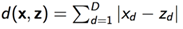
1)欧式距离
2)曼哈顿距离
3)余弦距离
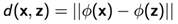
4)核函数映射后距离
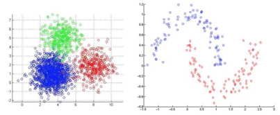
左边用欧氏距离,右边用核函数映射后距离:
层次聚类
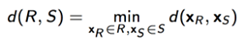
cluster R和cluster S之间的距离怎么界定?
① 最小连接距离法
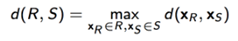
② 最大连接距离法
③ 平均连接距离法

聚类算法评价
1)purity评价法
purity方法是极为简单的一种聚类评价方法,只需计算正确聚类占总数的比例。
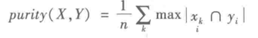
其中x = (x1, x2, x3…., xk)是聚类的集合,xk表示第k个聚类的集合。y = (y1, y2, y3…, yi)表示需要被聚合的集合,yi表示第i个聚类对象。n表示被聚合对象的总数。
2)RI评价法
实际上,这是一种用排列组合原理来对聚类进行评价的手段,RI评价公式如下
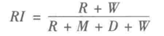
其中,R是指被聚在一类的两个对象被正确分类了,W是指不应该被聚在一类的两个对象被正确分开了,M指不应该放在一类的对象被错误的放在一类了,D指不应该分开的对象被错误的的分开了。
3)F值评价法
这是基于上述RI方法衍生出的一个方法,F评价公式如下。
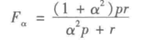
其中,
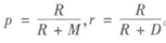
实际上RI方法就是把准确率p和召回率r看得同等重要,事实上,有时候我们可能需要某一特征更多一点,这时候就适合使用F值方法
K-means聚类
算法有三个步骤。第一步选择初始质心,给定最基本的方法是给定分类数k,从数据集中选择样本 X。初始化后,K-means由两个其他步骤之间的循环组成。第一步将每个样本分配到其最近的质心。第二步通过取分配给每个先前质心的所有样本的平均值来创建新的质心。计算旧和新质心之间的差异,并且算法重复这些最后两个步骤,直到该值小于阈值。换句话说,它重复,直到质心不显着移动。
这个算法是初始聚类中心敏感的,我们可以有一些办法缓解
1)初始第一个聚类中心为某个样本点,初始第二个聚类中心为离它最远的点,第三个为离它俩最远的…
2)多初始化几遍,选所有这些聚类中损失函数(到聚类中心和)最小的。
关于K的选定
很经典的“肘点”法:选取不同的K值;画出损失函数曲线;选取“肘点”值

K-means的局限性
1) 属于“硬聚类”,每个样本只能有一个类别。其他的一些聚类方法(GMM或者模糊K-means允许“软聚类”)
2) K-means对异常点的“免疫力”很差,我们可以通过一些调整(比如中心不直接取均值,而是找均值最近的样
本点代替)
3) 对于团状的数据点集区分度好,对于带状(环绕)等“非凸”形状不太好。(用谱聚类或者做特征映射
使用:
from sklearn.cluster import MiniBatchKMeans, KMeans
KMeans(n_clusters=8, init=’k-means++’, n_init=10, max_iter=300, tol=0.0001, precompute_distances=’auto’, verbose=0, random_state=None, copy_x=True, n_jobs=None, algorithm=’auto’)[source]
k_means.cluster_centers_
参数解释Parameters:
n_clusters : int, optional, default: 8
The number of clusters to form as well as the number of centroids to generate.
init : {‘k-means++’, ‘random’ or an ndarray}
Method for initialization, defaults to ‘k-means++’:
‘k-means++’ : selects initial cluster centers for k-mean clustering in a smart way to speed up convergence. See section Notes in k_init for more details.
‘random’: choose k observations (rows) at random from data for the initial centroids.
If an ndarray is passed, it should be of shape (n_clusters, n_features) and gives the initial centers.
n_init : int, default: 10
Number of time the k-means algorithm will be run with different centroid seeds. The final results will be the best output of n_init consecutive runs in terms of inertia.
max_iter : int, default: 300
Maximum number of iterations of the k-means algorithm for a single run.
tol : float, default: 1e-4
Relative tolerance with regards to inertia to declare convergence
precompute_distances : {‘auto’, True, False}
Precompute distances (faster but takes more memory).
‘auto’ : do not precompute distances if n_samples * n_clusters > 12 million. This corresponds to about 100MB overhead per job using double precision.
True : always precompute distances
False : never precompute distances
verbose : int, default 0
Verbosity mode.
random_state : int, RandomState instance or None (default)
Determines random number generation for centroid initialization. Use an int to make the randomness deterministic. See Glossary.
copy_x : boolean, optional
When pre-computing distances it is more numerically accurate to center the data first. If copy_x is True (default), then the original data is not modified, ensuring X is C-contiguous. If False, the original data is modified, and put back before the function returns, but small numerical differences may be introduced by subtracting and then adding the data mean, in this case it will also not ensure that data is C-contiguous which may cause a significant slowdown.
n_jobs : int or None, optional (default=None)
The number of jobs to use for the computation. This works by computing each of the n_init runs in parallel.
None means 1 unless in a joblib.parallel_backend context. -1 means using all processors. See Glossary for more details.
algorithm : “auto”, “full” or “elkan”, default=”auto”
K-means algorithm to use. The classical EM-style algorithm is “full”. The “elkan” variation is more efficient by using the triangle inequality, but currently doesn’t support sparse data. “auto” chooses “elkan” for dense data and “full” for sparse data.
Hierarchical clustering(层次聚类)
原理比较简单,这里简单说。从下往上不断形成簇,最开始将每个数据本身作为簇,然后将相邻最近的簇合并为一个簇,持续合并下去,直到满足一定条件。
使用:
AgglomerativeClustering(n_clusters=2, affinity=’euclidean’, memory=None, connectivity=None, compute_full_tree=’auto’, linkage=’ward’, pooling_func=’deprecated’)
参数解释arameters:
n_clusters : int, default=2
The number of clusters to find.
affinity : string or callable, default: “euclidean”
Metric used to compute the linkage. Can be “euclidean”, “l1”, “l2”, “manhattan”, “cosine”, or ‘precomputed’. If linkage is “ward”, only “euclidean” is accepted.
memory : None, str or object with the joblib.Memory interface, optional
Used to cache the output of the computation of the tree. By default, no caching is done. If a string is given, it is the path to the caching directory.
connectivity : array-like or callable, optional
Connectivity matrix. Defines for each sample the neighboring samples following a given structure of the data. This can be a connectivity matrix itself or a callable that transforms the data into a connectivity matrix, such as derived from kneighbors_graph. Default is None, i.e, the hierarchical clustering algorithm is unstructured.
compute_full_tree : bool or ‘auto’ (optional)
Stop early the construction of the tree at n_clusters. This is useful to decrease computation time if the number of clusters is not small compared to the number of samples. This option is useful only when specifying a connectivity matrix. Note also that when varying the number of clusters and using caching, it may be advantageous to compute the full tree.
linkage : {“ward”, “complete”, “average”, “single”}, optional (default=”ward”)
Which linkage criterion to use. The linkage criterion determines which distance to use between sets of observation. The algorithm will merge the pairs of cluster that minimize this criterion.
ward minimizes the variance of the clusters being merged.
average uses the average of the distances of each observation of the two sets.
complete or maximum linkage uses the maximum distances between all observations of the two sets.
single uses the minimum of the distances between all observations of the two sets.
pooling_func : callable, default=’deprecated’
DBSCAN(密度聚类)
给出一个邻域值r,对于一个样本点X,将与X样本点距离小于等于r的点都归为一个簇,然后遍历这个簇内所有的点,将与这些点距离小于等于r的数据都归为这个簇,循环执行这个过程。
使用:
DBSCAN(eps=0.5, min_samples=5, metric=’euclidean’, metric_params=None, algorithm=’auto’, leaf_size=30, p=None, n_jobs=None)
参数解释Parameters:
eps : float, optional
The maximum distance between two samples for them to be considered as in the same neighborhood.
min_samples : int, optional
The number of samples (or total weight) in a neighborhood for a point to be considered as a core point. This includes the point itself.
metric : string, or callable
The metric to use when calculating distance between instances in a feature array. If metric is a string or callable, it must be one of the options allowed by sklearn.metrics.pairwise_distances for its metric parameter. If metric is “precomputed”, X is assumed to be a distance matrix and must be square. X may be a sparse matrix, in which case only “nonzero” elements may be considered neighbors for DBSCAN.
New in version 0.17: metric precomputed to accept precomputed sparse matrix.
metric_params : dict, optional
Additional keyword arguments for the metric function.
New in version 0.19.
algorithm : {‘auto’, ‘ball_tree’, ‘kd_tree’, ‘brute’}, optional
The algorithm to be used by the NearestNeighbors module to compute pointwise distances and find nearest neighbors. See NearestNeighbors module documentation for details.
leaf_size : int, optional (default = 30)
Leaf size passed to BallTree or cKDTree. This can affect the speed of the construction and query, as well as the memory required to store the tree. The optimal value depends on the nature of the problem.
p : float, optional
The power of the Minkowski metric to be used to calculate distance between points.
n_jobs : int or None, optional (default=None)
The number of parallel jobs to run. None means 1 unless in a joblib.parallel_backend context. -1 means using all processors. See Glossary for more details.
kmodel.cluster_centers_ #查看聚类中心
kmodel.labels_ #查看各样本对应的类别
K-means VS 层次聚类 VS 高斯混合模型
① K-means这种扁平聚类产出一个聚类结果(都是独立的)
② 层次聚类能够根据你的聚类程度不同,有不同的结果
③ K-means需要指定聚类个数K,层次聚类不用
④ K-means比层次聚类要快一些(通常说来)
⑤ K-means用的多,可以用K- Median
高斯混合模型
1、优势
① 可理解性好:看做多个分布的组合
② 速度快:因为EM这种高效的算法在,时间复杂度O(tkn)
③ 学术上比较直观:最大数据似然概率
④ 其实可以拓展到多个其他分布的混合:多个多项式分布做类别判定
2、劣势
① 初始化要慎重,不然可能掉到局部最优里去
② 需要手工指定K(高斯分布)的个数
③ 对于我们提到的“非凸”分布数据集,也无能为力
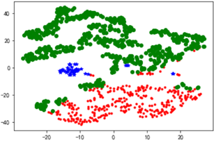
聚类结果可视化---TSNE
from sklearn.manifold import TSNE
tsne = TSNE()
tsne.fit_transform(data_zs) #进行数据降维
#tsne.embedding_是降维后的数据结果,维度是(n,2)
tsne = pd.DataFrame(tsne.embedding_, index = data_zs.index) #转换数据格式
import matplotlib.pyplot as plt
#不同类别用不同颜色和样式绘图
d = tsne[r[u'聚类类别'] == 0]
plt.plot(d[0], d[1], 'r.')
d = tsne[r[u'聚类类别'] == 1]
plt.plot(d[0], d[1], 'go')
d = tsne[r[u'聚类类别'] == 2]
plt.plot(d[0], d[1], 'b*')
plt.show()