一、鸢尾花种类预测
-
数据集分布
- load和fetch返回的数据类型datasets.base.Bunch(字典格式)
- data:特征数据数组,是 [n_samples * n_features] 的二维 numpy.ndarray 数组
- target:标签数组,是 n_samples 的一维 numpy.ndarray 数组
- DESCR:数据描述
- feature_names:特征名,新闻数据,手写数字、回归数据集没有
- target_names:标签名
-
数据集的划分
- 训练数据:用于训练,构建模型
- 测试数据:在模型检验时使用,用于评估模型是否有效
- 训练集:70% 80% 75%
- 测试集:30% 20% 25%
- 数据集划分api
- x 数据集的特征值
- y 数据集的标签值
- test_size 测试集的大小,一般为float
- random_state 随机数种子,不同的种子会造成不同的随机采样结果。相同的种子采样结果相同。
- return 测试集特征训练集特征值值,训练标签,测试标签(默认随机取)


# 内嵌绘图
import seaborn as sns
import matplotlib.pyplot as plt
import pandas as pd
from pylab import mpl
# 设置显示中文字体
mpl.rcParams["font.sans-serif"] = ["SimHei"]
from sklearn.datasets import load_iris,fetch_20newsgroups
from sklearn.model_selection import train_test_split
# 数据集获取
# 小数据集获取
iris = load_iris()
# print("鸢尾花数据集的返回值:
", iris)
# 返回值是一个继承自字典的Bench
# print("鸢尾花的特征值:
", iris["data"])
# print("鸢尾花的目标值:
", iris.target)
# print("鸢尾花特征的名字:
", iris.feature_names)
# print("鸢尾花目标值的名字:
", iris.target_names)
# print("鸢尾花的描述:
", iris.DESCR)
# Seaborn 是基于 Matplotlib 核心库进行了更高级的 API 封装,可以让你轻松地画出更漂亮的图形。而 Seaborn 的漂亮主要体现在配色更加舒服、以及图形元素的样式更加细腻。
# 安装 pip install seaborn
# seaborn.lmplot() 是一个非常有用的方法,它会在绘制二维散点图时,自动完成回归拟合
# sns.lmplot() 里的 x, y 分别代表横纵坐标的列名,
# data= 是关联到数据集,
# hue=*代表按照 species即花的类别分类显示,
# fit_reg=是否进行线性拟合。
# 把数据转换成dataframe的格式
iris_d = pd.DataFrame(iris['data'], columns=['Sepal_Length', 'Sepal_Width', 'Petal_Length', 'Petal_Width'])
iris_d['target'] = iris.target
# print(iris_d)
def plot_iris(iris,col1,col2 ):
sns.lmplot(x=col1, y=col2, data=iris, hue="target", fit_reg=False)
plt.xlabel(col1)
plt.ylabel(col2)
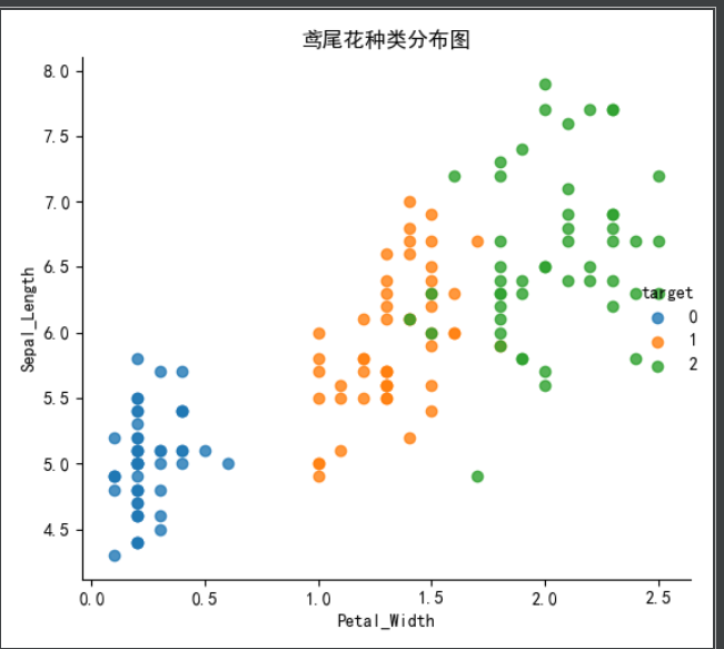
plt.title('鸢尾花种类分布图')
plt.show()
plot_iris(iris_d, 'Petal_Width', 'Sepal_Length')
plot_iris(iris_d, 'Petal_Width', 'Petal_Length')
# 训练集的划分
# 对鸢尾花数据集进行分割
# 训练集的特征值x_train 测试集的特征值x_test 训练集的目标值y_train 测试集的目标值y_test
x_train, x_test, y_train, y_test = train_test_split(iris.data, iris.target, random_state=22)
print("训练集的特征值x_train:
", x_train.shape)
print("测试集的特征值x_test:
", x_test.shape)
print("训练集的目标值y_train:
", y_train.shape)
print("测试集的目标值y_test:
", y_test.shape)
# 随机数种子
x_train1, x_test1, y_train1, y_test1 = train_test_split(iris.data, iris.target, random_state=6)
x_train2, x_test2, y_train2, y_test2 = train_test_split(iris.data, iris.target, random_state=6)
# print("如果随机数种子不一致:
", x_train == x_train1)
# print("如果随机数种子一致:
", x_train1 == x_train2)
进行模型预测的代码如下
from sklearn.datasets import load_iris
from sklearn.model_selection import train_test_split
from sklearn.preprocessing import StandardScaler
from sklearn.neighbors import KNeighborsClassifier

"""
1.获取数据集
2.数据基本处理
3.特征工程
4.机器学习(模型训练)
5.模型评估
"""
# 1.获取数据集
iris = load_iris()

# 2.数据基本处理
# 2.1 数据分割
x_train, x_test, y_train, y_test = train_test_split(iris.data, iris.target, random_state=22, test_size=0.2)

# 3.特征工程
# 3.1 实例化一个转换器
transfer = StandardScaler()
# 3.2 调用fit_transform方法
x_train = transfer.fit_transform(x_train)
x_test = transfer.fit_transform(x_test)

# 4.机器学习(模型训练)
# 4.1 实例化一个估计器
estimator = KNeighborsClassifier(n_neighbors=5)
# 4.2 模型训练
estimator.fit(x_train, y_train)

# 5.模型评估
# 5.1 输出预测值
y_pre = estimator.predict(x_test)
print("预测值是:
", y_pre)
print("预测值和真实值对比:
", y_pre == y_test)

# 5.2 输出准确率
ret = estimator.score(x_test, y_test)
print("准确率是:
", ret)

我们可以看出这样预测的准确率并不高,所以就要对算法进行优化,提高预测的准确率,就要用到下面的交叉验证和网格搜索的方法
-
交叉验证,网格搜索
什么是交叉验证(cross validation)
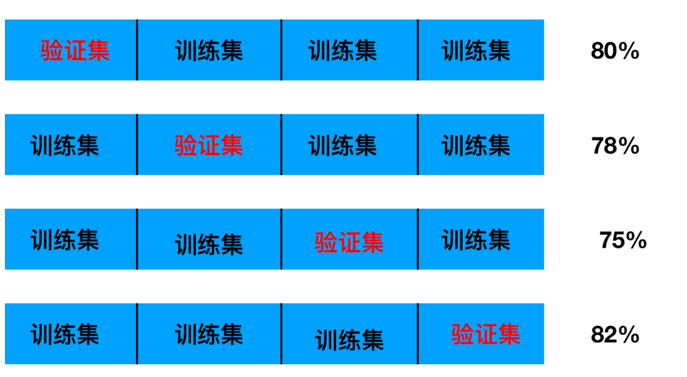
交叉验证:将拿到的训练数据,分为训练和验证集。以下图为例:将数据分成4份,其中一份作为验证集。然后经过4次(组)的测试,每次都更换不同的验证集。即得到4组模型的结果,取平均值作为最终结果。又称4折交叉验证。
数据分为训练集和测试集,但是为了让从训练得到模型结果更加准确。做以下处理 -
训练集:训练集+验证集
-
测试集:测试集
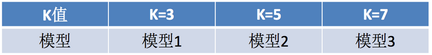
什么是网格搜索(Grid Search)
通常情况下,有很多参数是需要手动指定的(如k-近邻算法中的K值),这种叫超参数。但是手动过程繁杂,所以需要对模型预设几种超参数组合。每组超参数都采用交叉验证来进行评估。最后选出最优参数组合建立模型。
- sklearn.model_selection.GridSearchCV(estimator, param_grid=None,cv=None)
- 对估计器的指定参数值进行详尽搜索
- estimator:估计器对象
- param_grid:估计器参数(dict){“n_neighbors”:[1,3,5]}
- cv:指定几折交叉验证
- fit:输入训练数据
- score:准确率
- 结果分析:
- bestscore__:在交叉验证中验证的最好结果
- bestestimator:最好的参数模型
- cvresults:每次交叉验证后的验证集准确率结果和训练集准确率结果
调优后的代码
"""
1.获取数据集
2.数据基本处理
3.特征工程
4.机器学习(模型训练)
5.模型评估
"""
from sklearn.datasets import load_iris
from sklearn.model_selection import train_test_split, GridSearchCV
from sklearn.preprocessing import StandardScaler
from sklearn.neighbors import KNeighborsClassifier
if __name__=='__main__':
# 1.获取数据集
iris = load_iris()
# 2.数据基本处理
# 2.1 数据分割
x_train, x_test, y_train, y_test = train_test_split(iris.data, iris.target, test_size=0.2)
# 3.特征工程
# 3.1 实例化一个转换器
transfer = StandardScaler()
# 3.2 调用fit_transform方法
x_train = transfer.fit_transform(x_train)
x_test = transfer.fit_transform(x_test)
# 4.机器学习(模型训练)
# 4.1 实例化一个估计器
estimator = KNeighborsClassifier()
# 4.2 调用交叉验证网格搜索模型
param_grid = {"n_neighbors": [1, 3, 5, 7, 9]}
estimator = GridSearchCV(estimator, param_grid=param_grid, cv=10, n_jobs=-1)
# 4.3 模型训练
estimator.fit(x_train, y_train)
# 5.模型评估
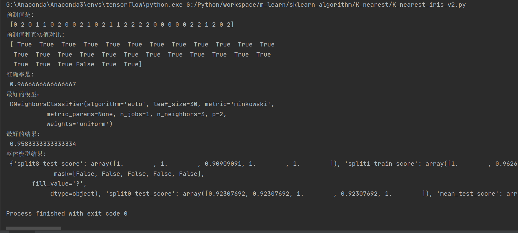
# 5.1 输出预测值
y_pre = estimator.predict(x_test)
print("预测值是:
", y_pre)
print("预测值和真实值对比:
", y_pre == y_test)
# 5.2 输出准确率
ret = estimator.score(x_test, y_test)
print("准确率是:
", ret)
# 5.3 其他评价指标
print("最好的模型:
", estimator.best_estimator_)
print("最好的结果:
", estimator.best_score_)
print("整体模型结果:
", estimator.cv_results_)
二、预测facebook签到位置
数据介绍:将根据用户的位置,准确性和时间戳预测用户正在查看的业务。
train.csv,test.csv
row_id:登记事件的ID
xy:坐标
准确性:定位准确性
时间:时间戳
place_id:业务的ID,这是您预测的目标
- 步骤分析
-
对于数据做一些基本处理(这里所做的一些处理不一定达到很好的效果,我们只是简单尝试,有些特征我们可以根据一些特征选择的方式去做处理)
-
1 缩小数据集范围 DataFrame.query()
-
2 选取有用的时间特征
-
3 将签到位置少于n个用户的删除
-
-
分割数据集
-
标准化处理
-
k-近邻预测
-
本数据集的数据较多

代码
import pandas as pd

from sklearn.model_selection import train_test_split, GridSearchCV
from sklearn.preprocessing import StandardScaler
from sklearn.neighbors import KNeighborsClassifier

facebook = pd.read_csv("../../data/train.csv")

# 2.基本数据处理
# 2.1 缩小数据范围
facebook_data = facebook.query("x>2.0 & x<2.5 & y>2.0 & y<2.5")
# 2.2 选择时间特征
time = pd.to_datetime(facebook_data["time"], unit="s")
time = pd.DatetimeIndex(time)
facebook_data["day"] = time.day
facebook_data["hour"] = time.hour
facebook_data["weekday"] = time.weekday
# 2.3 去掉签到较少的地方
place_count = facebook_data.groupby("place_id").count()
place_count = place_count[place_count["row_id"]>3]
facebook_data = facebook_data[facebook_data["place_id"].isin(place_count.index)]
# 2.4 确定特征值和目标值
x = facebook_data[["x", "y", "accuracy", "day", "hour", "weekday"]]
y = facebook_data["place_id"]
# 2.5 分割数据集
x_train, x_test, y_train, y_test = train_test_split(x, y, random_state=22)

# 3.特征工程--特征预处理(标准化)
# 3.1 实例化一个转换器
transfer = StandardScaler()
# 3.2 调用fit_transform
x_train = transfer.fit_transform(x_train)
x_test = transfer.fit_transform(x_test)

# 4.机器学习--knn+cv
# 4.1 实例化一个估计器
estimator = KNeighborsClassifier()
# 4.2 调用gridsearchCV
param_grid = {"n_neighbors": [1, 3, 5, 7, 9]}
estimator = GridSearchCV(estimator, param_grid=param_grid, cv=5)
# 4.3 模型训练
estimator.fit(x_train, y_train)

# 5.模型评估
# 5.1 基本评估方式
score = estimator.score(x_test, y_test)
print("最后预测的准确率为:
", score)

y_predict = estimator.predict(x_test)
print("最后的预测值为:
", y_predict)
print("预测值和真实值的对比情况:
", y_predict == y_test)

# 5.2 使用交叉验证后的评估方式
print("在交叉验证中验证的最好结果:
", estimator.best_score_)
print("最好的参数模型:
", estimator.best_estimator_)
print("每次交叉验证后的验证集准确率结果和训练集准确率结果:
",estimator.cv_results_)
因为数据量较大,即使已经做过了数据截取,依然需要运行几分钟的时间,请耐心等待
