HEC-ResSim原文档

HEC-ResSim

Reservoir System Simulation

User's Manual

Version 3.1 May 2013

Approved for Public Release. Distribution Unlimited. CPD-82

REPORT DOCUMENTATION PAGE

Form Approved OMB No. 0704-0188

The public reporting burden for this collection of information is estimated to average 1 hour per response, including the time for reviewing instructions, searching existing data sources, gathering and maintaining the data needed, and completing and reviewing the collection of information. Send comments regarding this burden estimate or any other aspect of this collection of information, including suggestions for reducing this burden, to the Department of Defense, Executive Services and Communications Directorate (0704-0188). Respondents should be aware that notwithstanding any other provision of law, no person shall be subject to any penalty for failing to comply with a collection of information if it does not display a currently valid OMB control number.

PLEASE DO NOT RETURN YOUR FORM TO THE ABOVE ORGANIZATION.

1. REPORT DATE (DD-MM-YYYY)

May 2013

2. REPORT TYPE

Computer Program Documentation

3. DATES COVERED (From - To)

4. TITLE AND SUBTITLE

HEC-ResSim

Reservoir System Simulation User's Manual

Version 3.1

5a. CONTRACT NUMBER

5b. GRANT NUMBER

5c. PROGRAM ELEMENT NUMBER

6. AUTHOR(S)

Joan D. Klipsch

Marilyn B. Hurst

5d. PROJECT NUMBER

5e. TASK NUMBER

5F. WORK UNIT NUMBER

7. PERFORMING ORGANIZATION NAME(S) AND ADDRESS(ES)

US Army Corps of Engineers

Institute for Water Resources

Hydrologic Engineering Center (HEC)

609 Second Street

Davis, CA 95616-4687

8. PERFORMING ORGANIZATION REPORT NUMBER

CPD-82

9. SPONSORING/MONITORING AGENCY NAME(S) AND ADDRESS(ES)

10. SPONSOR/ MONITOR'S ACRONYM(S)

11. SPONSOR/ MONITOR'S REPORT NUMBER(S)

12. DISTRIBUTION / AVAILABILITY STATEMENT

Approved for public release; distribution is unlimited.

13. SUPPLEMENTARY NOTES

Also, see HEC-ResSim Quick Start Guide, CPD-82a

14. ABSTRACT

The U.S. Army Corps of Engineers' Hydrologic Engineering Center's Reservoir System Simulation (HECResSim) is a computer program comprised of a graphical user interface (GUI) and a computational program to simulate reservoir operations. Included are data storage and management capabilities and graphics and reporting facilities. HEC's Data Storage System (HEC-DSS) is used for storage and retrieval of input and output time series data.

15. SUBJECT TERMS

HEC-ResSim, Reservoir Simulation, computer program

16. SECURITY CLASSIFICATION OF:

17. LIMITATION

OF ABSTRACT

18. NUMBER

OF PAGES

556

19a. NAME OF RESPONSIBLE PERSON

a. REPORT

b. ABSTRACT

c. THIS PAGE

19b. TELEPHONE NUMBER

Standard Form 298 (Rev. 8/98) Prescribed by ANSI Std. Z39-18

HEC-ResSim

Reservoir System Simulation

User's Manual

Version 3.1 May 2013

US Army Corps of Engineers

Institute for Water Resources

Hydrologic Engineering Center

609 Second Street

Davis, CA 95616

(530) 756-1104 (530) 756-8250 FAX

www.hec.usace.army.mil CPD-82 Reservoir System Simulation, HEC-ResSim

Software Distribution and Support Statement:

2013. This Hydrologic Engineering Center (HEC) documentation was developed with U.S. Federal Government resources and is therefore in the public domain. It may be used, copied, distributed, or redistributed freely. However, it is requested that HEC be given appropriate acknowledgment in any subsequent use of this work.

Use of the software described by this document is controlled by certain terms and conditions. The user must acknowledge and agree to be bound by the terms and conditions of usage before the software can be installed or used. For reference, a copy of the terms and conditions of usage are included below so that they may be examined before obtaining the software. The software described by this document can be downloaded for free from our internet site (www.hec.usace.army.mil ).

HEC cannot provide technical support for this software to non-Corps users. See our software vendor list (on our web page) to locate organizations that provide the program, documentation, and support services for a fee. However, we will respond to all documented instances of program errors. Documented errors are bugs in the software due to programming mistakes not model problems due to user-entered data.

This document contains references to product names that are trademarks or registered trademarks of their respective owners. Use of specific product names does not imply official or unofficial endorsement. Product names are used solely for the purpose of identifying products available in the public market place.

Microsoft and Windows are registered trademarks of Microsoft Corp. Solaris and Java are trademarks of Sun Microsystems, Inc.

Terms and Conditions for Use of HEC-ResSim:

The United States Government, US Army Corps of Engineers, Hydrologic Engineering Center ("HEC") grants to the user the rights to install HECResSim "the Software" (either from a disk copy obtained from HEC, a distributor or another user or by downloading it from a network) and to use, copy and/or distribute copies of the Software to other users, subject to the following Terms and Conditions of Use:

All copies of the Software received or reproduced by or for user pursuant to the authority of this Terms and Conditions of Use will be and remain the property of HEC.

User may reproduce and distribute the Software provided that the recipient agrees to the Terms and Conditions for Use noted herein.

HEC is solely responsible for the content of the Software. The Software may not be modified, abridged, decompiled, disassembled, unobfuscated or reverse engineered. The user is solely responsible for the content, interactions, and effects of any and all amendments, if present, whether they be extension modules, language resource bundles, scripts or any other amendment.

No part of this Terms and Conditions for Use may be modified, deleted or obliterated from the Software.

No part of the Software may be exported or re-exported in contravention of U.S. export laws or regulations.

Waiver of Warranty

THE UNITED STATES GOVERNMENT AND ITS AGENCIES, OFFICIALS, REPRESENTATIVES, AND EMPLOYEES, INCLUDING ITS

CONTRACTORS AND SUPPLIERS PROVIDE HEC-RESSIM "AS IS," WITHOUT ANY WARRANTY OR CONDITION, EXPRESS, IMPLIED OR

STATUTORY, AND SPECIFICALLY DISCLAIM ANY IMPLIED WARRANTIES OF TITLE, MERCHANTABILITY, FITNESS FOR A PARTICULAR

PURPOSE AND NON-INFRINGEMENT. Depending on state law, the foregoing disclaimer may not apply to you, and you may also have other legal rights that vary from state to state.

Limitation of Liability

IN NO EVENT SHALL THE UNITED STATES GOVERNMENT AND ITS AGENCIES, OFFICIALS, REPRESENTATIVES, AND EMPLOYEES,

INCLUDING ITS CONTRACTORS AND SUPPLIERS, BE LIABLE FOR LOST PROFITS OR ANY SPECIAL, INCIDENTAL OR CONSEQUENTIAL DAMAGES ARISING OUT OF OR IN CONNECTION WITH USE OF HEC-RESSIM REGARDLESS OF CAUSE, INCLUDING NEGLIGENCE.

THE UNITED STATES GOVERNMENT'S LIABILITY, AND THE LIABILITY OF ITS AGENCIES, OFFICIALS, REPRESENTATIVES, AND

EMPLOYEES, INCLUDING ITS CONTRACTORS AND SUPPLIERS, TO YOU OR ANY THIRD PARTIES IN ANY CIRCUMSTANCE IS LIMITED TO THE REPLACEMENT OF CERTIFIED COPIES OF HEC-RESSIM WITH IDENTIFIED ERRORS CORRECTED. Depending on state law, the above limitation or exclusion may not apply to you.

Indemnity

As a voluntary user of HEC-ResSim you agree to indemnify and hold the United States Government, and its agencies, officials, representatives, and employees, including its contractors and suppliers, harmless from any claim or demand, including reasonable attorneys' fees, made by any third party due to or arising out of your use of HEC-ResSim or breach of this Agreement or your violation of any law or the rights of a third party.

Assent

By using this program you voluntarily accept these terms and conditions. If you do not agree to these terms and conditions, uninstall the program and return any program materials to HEC (If you downloaded the program and do not have disk media, please delete all copies, and cease using the program).

HEC-ResSim User's Manual

Page

LIST OF APPENDICES ............................................................................................. X

LIST OF TABLES ...................................................................................................... X

LIST OF FIGURES ................................................................................................... XI

HISTORY AND ACKNOWLEDGMENTS ................................................................ XXV

Chapter Page

1 INTRODUCTION .................................................................................................... 1-1

1.1 RESSIM MODULES ...........................................................................................1 -1

1.1.1 WATERSHED SETUP MODULE ............................................................... 1-2

1.1.2 RESERVOIR NETWORK MODULE ............................................................ 1-2

1.1.3 SIMULATION MODULE ........................................................................... 1-3

1.2 ABOUT THIS MANUAL .......................................................................................1 -3

2 RESSIM CONCEPTS ............................................................................................. 2-1

2.1 STARTING RESSIM ..........................................................................................2 -2

2.2 RECOGNIZING COMMON SCREEN COMPONENTS................................................ 2-3

2.2.1 MENU BAR........................................................................................... 2-3

2.2.2 MODULE LIST ....................................................................................... 2-5

2.3 WATERSHED SETUP MODULE ...........................................................................2 -6

2.4 RESERVOIR NETWORK MODULE ..................................................................... 2-10

2.5 SIMULATION MODULE..................................................................................... 2-13

2.6 OPENING AN EXISTING WATERSHED ............................................................... 2-15

2.7 UNDERSTANDING SCHEMATIC ELEMENTS ........................................................ 2-17

2.7.1 STREAM ALIGNMENT .......................................................................... 2-17

2.7.2 OTHER WATERSHED ELEMENTS ......................................................... 2-17

2.7.3 RESERVOIR NETWORK SCHEMATIC ..................................................... 2-19

2.7.4 USING SHORTCUT MENUS .................................................................. 2-20

2.8 PRINTING AND EXPORTING REPORTS ............................................................. 2-20

2.8.1 PRINTING REPORTS ........................................................................... 2-21

2.8.2 PRINT PREVIEW ................................................................................. 2-24

2.8.3 EXPORTING REPORTS TO A FILE ........................................................ 2-25

3 CREATING AND MANAGING WATERSHEDS ..................................................... 3-1

3.1 RECOGNIZING WATERSHED SETUP SCREEN COMPONENTS ................................ 3-1

3.1.1 MENU BAR........................................................................................... 3-2 3.1.2 CONFIGURATION SELECTOR AND LOCK/UNLOCK .................................... 3-4 3.1.3 MAP (MOUSE) TOOLS ........................................................................... 3-4

3.2 USING SHORTCUT MENUS ................................................................................3 -6 3.3 WATERSHED CREATION ...................................................................................3 -6

3.3.1 DEFINING A WATERSHED LOCATION ...................................................... 3-6 3.3.2 CREATING A NEW WATERSHED ............................................................. 3-8 3.3.3 SPECIFYING UNITS OF MEASURE .......................................................... 3-9 3.3.4 SPECIFYING TIME ZONE........................................................................ 3-9

3.4 SETTING UP NEW MAP LAYERS ........................................................................3 -9

3.4.1 IMPORTING MAPS INTO RESSIM ............................................................ 3-9 3.4.2 ADDING A NEW MAP LAYER ................................................................ 3-12

3.4.3 SPECIFYING THE GEOGRAPHIC REFERENCING AND

COORDINATE SYSTEM ................................................................... 3-13

4 WORKING WITH LAYERS .................................................................................... 4-1

4.1 UNDERSTANDING LAYERS ................................................................................4 -1

4.1.1 TIME-SERIES ICON LAYER .................................................................... 4-1

4.1.2 STUDY LAYER ...................................................................................... 4-1

4.1.3 STREAM ALIGNMENT LAYER .................................................................. 4-2

4.1.4 MAP LAYERS ....................................................................................... 4-2

4.2 EXPLORING THE LAYER SELECTOR ...................................................................4 -2

4.2.1 THE LAYER SELECTOR MENUS ............................................................. 4-3

4.2.2 THE LAYER SELECTOR "TREE" .............................................................. 4-4

4.2.3 CONTROLLING LAYER DISPLAY ............................................................. 4-5

4.2.4 VIEWING LAYER LEGEND ...................................................................... 4-6

4.3 CONTROLLING LAYER ORGANIZATION ...............................................................4 -6

4.3.1 CONFIGURING TOOLBAR ICONS TO CONTROL LAYERS ............................ 4-7

4.3.2 ADDING MAP LAYERS ........................................................................... 4-8

4.3.3 REMOVING MAP LAYERS ...................................................................... 4-8

4.3.4 USING LAYER SELECTOR SHORTCUT MENUS ......................................... 4-9

4.4 VIEWING AND CONFIGURING LAYER PROPERTIES ............................................ 4-10

4.4.1 STUDY LAYER PROPERTIES ................................................................ 4-11

4.4.2 STREAM ALIGNMENT LAYER PROPERTIES ............................................ 4-15

4.4.3 MAP LAYERS PROPERTIES .................................................................. 4-16

5 WORKING WITH THE STREAM ALIGNMENT ...................................................... 5-1

5.1 CREATING A NEW STREAM ALIGNMENT .............................................................5 -2

5.2 EDITING AN EXISTING STREAM ALIGNMENT ....................................................... 5-5

5.2.1 MOVING VERTICES OF A STREAM ELEMENT ........................................... 5-5

5.2.2 ADDING VERTICES TO A STREAM ELEMENT ............................................ 5-6

5.2.3 DELETING VERTICES FROM A STREAM ELEMENT .................................... 5-6

5.2.4 EDITING A STREAM ELEMENT ................................................................ 5-6

5.2.5 RENAMING A STREAM ELEMENT ............................................................ 5-8

5.2.6 DELETING A STREAM ELEMENT ............................................................. 5-8

5.2.7 INSERTING A STREAM NODE ................................................................. 5-9

5.2.8 EDITING A STREAM NODE ..................................................................... 5-9

5.2.9 DELETING A STREAM NODE ................................................................ 5-10

5.2.10 MOVING A STREAM JUNCTION ............................................................. 5-10

5.2.11 EDITING A STREAM JUNCTION ............................................................. 5-11

5.2.12 REVERSING THE DIRECTION OF A STREAM ........................................... 5-11

5.2.13 DISCONNECTING A STREAM ELEMENT ................................................. 5-12

5.3 IMPORTING A STREAM ALIGNMENT .................................................................. 5-12

5.4 EXPORTING A STREAM ALIGNMENT ................................................................. 5-14

5.5 CONFIGURING STREAM ALIGNMENT DISPLAY PROPERTIES ............................... 5-15

5.6 SAVING THE STREAM ALIGNMENT ................................................................... 5-16

5.7 LISTING OF STREAMS ..................................................................................... 5-16

6 CREATING WATERSHED ELEMENTS ................................................................. 6-1

6.1 CREATING A RESERVOIR ..................................................................................6 -1

6.1.1 EDITING RESERVOIR DATA (WATERSHED SETUP) .................................. 6-2

6.1.2 RENAMING A RESERVOIR ...................................................................... 6-3

6.1.3 REMOVING A RESERVOIR FROM A CONFIGURATION ................................ 6-4

6.1.4 DELETING A RESERVOIR ....................................................................... 6-4

6.1.5 ADDING CONFIGURATION NOTES FOR A RESERVOIR............................... 6-4

6.2 CREATING A LEVEE ..........................................................................................6 -5

6.2.1 EDITING LEVEE DATA ........................................................................... 6-5

6.2.2 RENAMING A LEVEE.............................................................................. 6-7

6.2.3 REMOVING A LEVEE FROM A CONFIGURATION ........................................ 6-7

6.2.4 DELETING A LEVEE ............................................................................... 6-8

6.2.5 ADDING CONFIGURATION NOTES FOR A LEVEE ...................................... 6-8

6.3 CREATING A DIVERSION ...................................................................................6 -9

6.3.1 EDITING DIVERSION DATA .................................................................. 6-10

6.3.2 RENAMING A DIVERSION ..................................................................... 6-10

6.3.3 DISCONNECTING A DIVERSION ............................................................ 6-11

6.3.4 REMOVING A DIVERSION FROM A CONFIGURATION ............................... 6-11

6.3.5 DELETING A DIVERSION ...................................................................... 6-11

6.3.6 ADDING CONFIGURATION NOTES FOR A DIVERSION .............................. 6-12

6.4 CREATING CHANNEL MODIFICATIONS .............................................................. 6-12

6.4.1 EDITING CHANNEL MODIFICATION DATA .............................................. 6-12

6.4.2 RENAMING A CHANNEL MODIFICATION ................................................. 6-13

6.4.3 REMOVING A CHANNEL MODIFICATION FROM A CONFIGURATION ........... 6-14

6.4.4 DELETING A CHANNEL MODIFICATION .................................................. 6-14

6.4.5 ADDING CONFIGURATION NOTES FOR CHANNEL MODIFICATIONS .......... 6-14

6.5 CREATING OFF-CHANNEL STORAGE AREAS .................................................... 6-15

6.5.1 EDITING OFF-CHANNEL STORAGE DATA .............................................. 6-15

6.5.2 RENAMING AN OFF-CHANNEL STORAGE AREA ..................................... 6-16

6.5.3 REMOVING AN OFF-CHANNEL STORAGE AREA FROM

A CONFIGURATION ........................................................................ 6-16

6.5.4 DELETING AN OFF-CHANNEL STORAGE AREA ...................................... 6-17

6.5.5 ADDING CONFIGURATION NOTES FOR AN

OFF-CHANNEL STORAGE AREA ..................................................... 6-17

6.6 CREATING "OTHER" PROJECTS....................................................................... 6-18

6.6.1 EDITING "OTHER" PROJECT DATA ....................................................... 6-18 6.6.2 RENAMING "OTHER" PROJECTS .......................................................... 6-19

6.6.3 REMOVING "OTHER" PROJECTS FROM A CONFIGURATION ..................... 6-19

6.6.4 DELETING "OTHER" PROJECTS ........................................................... 6-20

6.6.5 ADDING CONFIGURATION NOTES FOR "OTHER" PROJECTS ................... 6-20

6.7 CONFIGURING PROJECT DISPLAY PROPERTIES ............................................... 6-20 6.8 DEFINING COMPUTATION POINTS ................................................................... 6-21

6.8.1 EDITING COMPUTATION POINT DATA ................................................... 6-21

6.8.2 RENAMING A COMPUTATION POINT AND EDITING THE DESCRIPTION ...... 6-23

6.8.3 DELETING A COMPUTATION POINT ...................................................... 6-23

6.9 WORKING WITH TIME-SERIES ICONS ............................................................... 6-24

7 CREATING WATERSHED CONFIGURATIONS .................................................... 7-1

7.1 ADDING WATERSHED CONFIGURATIONS ...........................................................7 -1

7.2 ADDING AND REMOVING PROJECTS FROM CONFIGURATIONS ............................. 7-3

7.2.1 ADDING PROJECTS TO A CONFIGURATION ............................................. 7-4

7.2.2 REMOVING PROJECTS FROM A CONFIGURATION .................................... 7-4

7.3 ADDING PROJECT NOTES TO A CONFIGURATION ................................................ 7-5

7.4 MAKING A COPY OF A CONFIGURATION ............................................................. 7-5

7.5 DELETING A CONFIGURATION ...........................................................................7 -6

7.6 SAVING CONFIGURATION DATA.........................................................................7 -6

7.7 LISTING CONFIGURATIONS ...............................................................................7 -6

8 DEVELOPING A RESERVOIR NETWORK ........................................................... 8-1

8.1 RECOGNIZING RESERVOIR NETWORK SCREEN COMPONENTS ............................ 8-2

8.1.1 MENU BAR........................................................................................... 8-3

8.1.2 NETWORK, CONFIGURATION, AND LOCK/UNLOCK ................................... 8-5

8.1.3 MAP (MOUSE) TOOLS ........................................................................... 8-5

8.1.4 DISPLAY AREA ..................................................................................... 8-6

8.2 DEFINING A RESERVOIR NETWORK ...................................................................8 -7

8.2.1 CREATING A NEW RESERVOIR NETWORK .............................................. 8-7

8.2.2 OPENING AN EXISTING RESERVOIR NETWORK ....................................... 8-8

8.2.3 IMPORTING A RESERVOIR NETWORK ..................................................... 8-9 _New

8.3 MAKING THE NETWORK EDITABLE ................................................................... 8-12

8.4 ADDING ROUTING REACHES ........................................................................... 8-12

8.4.1 DRAWING ROUTING REACHES............................................................. 8-12

8.4.2 RENAMING ROUTING REACHES ........................................................... 8-13

8.4.3 DELETING ROUTING REACHES ............................................................ 8-14

8.5 VIEWING NETWORK REPORTS ........................................................................ 8-14

8.5.1 VIEWING THE RESERVOIR LIST ............................................................ 8-14

8.5.2 VIEWING THE REACH LIST ................................................................... 8-15

8.5.3 VIEWING THE JUNCTION LIST .............................................................. 8-15

8.5.4 VIEWING THE DIVERSION LIST ............................................................. 8-16

8.5.5 VIEWING ADVANCED REPORTS ........................................................... 8-17

8.6 UPDATING A RESERVOIR NETWORK ................................................................ 8-19

9 EDITING JUNCTION, REACH, AND DIVERSION DATA ...................................... 9-1

9.1 EDITING JUNCTION PROPERTIES .......................................................................9 -1

9.1.1 JUNCTION EDITOR: INFO TAB ............................................................... 9-2

9.1.2 JUNCTION EDITOR: LOCAL FLOW TAB ................................................... 9-3

9.1.3 JUNCTION EDITOR: RATING CURVE TAB ................................................ 9-4

9.1.4 JUNCTION EDITOR: OBSERVED DATA TAB ............................................. 9-5

9.2 EDITING REACH PROPERTIES ...........................................................................9 -6

9.2.1 REACH EDITOR: ROUTING TAB ............................................................. 9-7

9.2.2 REACH EDITOR: LOSSES TAB ............................................................. 9-18

9.2.3 REACH EDITOR: OBSERVED DATA TAB ............................................... 9-18

9.3 EDITING DIVERSION PROPERTIES ................................................................... 9-19

9.3.1 DIVERSION EDITOR: DIVERSION TAB ................................................... 9-20

9.3.2 DIVERSION EDITOR: ROUTING TAB ..................................................... 9-33

9.3.3 DIVERSION EDITOR: LOSSES TAB ....................................................... 9-33

9.3.4 DIVERSION EDITOR: OBSERVED DATA TAB ......................................... 9-34

10 DEFINING PHYSICAL COMPONENTS OF RESERVOIRS .............................. 10-1

10.1 ACCESSING THE RESERVOIR EDITOR ........................................................ 10-2

10.2 USING THE RESERVOIR EDITOR TO DEFINE PHYSICAL COMPONENTS .......... 10-2

10.3 SPECIFYING PHYSICAL COMPONENTS OF A RESERVOIR ............................. 10-3

10.4 SPECIFYING RESERVOIR POOL LOSSES .................................................... 10-4

10.5 DEFINING PHYSICAL FEATURES OF A DAM ................................................. 10-4

10.6 ADDING LEAKAGE TO A DAM ..................................................................... 10-5

10.7 ADDING OUTLET GROUPS ........................................................................ 10-6

10.8 DEFINING CONTROLLED OUTLETS ............................................................. 10-7

10.8.1 ADDING CONTROLLED OUTLETS ................................................. 10-7

10.8.2 ADDING POWER PLANTS ............................................................ 10-8

10.8.3 ADDING PUMPS ......................................................................... 10-9

10.9 ADDING UNCONTROLLED OUTLETS ......................................................... 10-10

10.10 ADDING TAILWATER ELEVATION .............................................................. 10-11

10.11 DEFINING PHYSICAL COMPONENTS OF A DIVERTED OUTLET ..................... 10-12

10.12 RENAMING, DELETING, AND REMOVING RESERVOIR COMPONENTS ........... 10-13

10.12.1 RENAMING RESERVOIR COMPONENTS ...................................... 10-13

10.12.2 DELETING RESERVOIR COMPONENTS ....................................... 10-14

10.12.3 REMOVING RESERVOIR PARAMETERS....................................... 10-15

10.13 EDITING RESERVOIR PHYSICAL DATA ...................................................... 10-15

10.14 EDITING POOL PHYSICAL DATA ............................................................... 10-16

10.14.1 EDITING POOL EVAPORATION DATA .......................................... 10-17

10.14.2 EDITING POOL SEEPAGE .......................................................... 10-18

10.15 EDITING DAM LEAKAGE .......................................................................... 10-19

10.16 EDITING CONTROLLED OUTLET PHYSICAL DATA ...................................... 10-20

10.17 EDITING POWER PLANT PHYSICAL DATA ................................................. 10-22

10.17.1 EDITING OUTLET CAPACITY DATA FOR A POWER PLANT ............ 10-22

10.17.2 EDITING CAPACITY DATA FOR A POWER PLANT ......................... 10-23 10.17.3 EDITING EFFICIENCY DATA FOR A POWER PLANT ...................... 10-26 10.17.4 EDITING STATION USE DATA FOR A POWER PLANT .................... 10-30

10.17.5 EDITING HYDRAULIC LOSSES DATA FOR A POWER PLANT .......... 10-32

10.18 EDITING PUMP PHYSICAL DATA .............................................................. 10-34

10.18.1 PUMP CAPACITY AS CONSTANT ................................................ 10-34

10.18.2 PUMP CAPACITY AS FUNCTION OF OPERATING HEAD ................ 10-35

10.19 EDITING UNCONTROLLED OUTLET PHYSICAL DATA .................................. 10-36 10.20 EDITING TAILWATER ELEVATION PHYSICAL DATA ..................................... 10-37

10.21 VIEWING COMPOSITE RELEASE CAPACITY TABLES .................................. 10-39

10.21.1 RESERVOIR COMPOSITE RELEASE CAPACITY TABLE ................. 10-39

10.21.2 DAM COMPOSITE RELEASE CAPACITY TABLE ............................ 10-40

10.21.3 DIVERTED OUTLET COMPOSITE RELEASE CAPACITY TABLE ....... 10-40 10.21.4 OUTLET GROUP COMPOSITE RELEASE CAPACITY TABLE ........... 10-40

10.22 RESERVOIR EDITOR: PULSE FLOW OPTIONS ........................................... 10-41 10.23 RESERVOIR EDITOR: OBSERVED DATA TAB ............................................ 10-42

11 DEFINING RESERVOIR OPERATIONS DATA ................................................ 11-1

11.1 RESERVOIR EDITOR'S OPERATIONS TAB ................................................... 11-2 11.2 RESERVOIR OPERATION SETS .................................................................. 11-3

11.2.1 CREATING A NEW OPERATION SET ............................................. 11-3 11.2.2 RENAMING AN OPERATION SET .................................................. 11-4 11.2.3 COPYING AN OPERATION SET .................................................... 11-5 11.2.4 DELETING AN OPERATION SET ................................................... 11-5 11.2.5 EDITING AN OPERATION SET ...................................................... 11-6

11.3 RESERVOIR OPERATION ZONES ................................................................ 11-6

11.3.1 RENAMING AND DESCRIBING OPERATION ZONES......................... 11-7 11.3.2 ADDING A NEW RESERVOIR STORAGE ZONE ............................... 11-7 11.3.3 DEFINING OPERATION ZONES .................................................... 11-8 11.3.4 DELETING OPERATION ZONES .................................................. 11-13

11.4 UNDERSTANDING RESERVOIR OPERATION RULES ................................... 11-14

11.4.1 RELEASE DECISION PROCESS .................................................. 11-14 11.4.2 USING EXISTING RULES ........................................................... 11-14 11.4.3 REMOVING RULES ................................................................... 11-15 11.4.4 DELETING RULES .................................................................... 11-15 11.4.5 PRIORITIZING RULES ............................................................... 11-15 11.4.6 RENAMING RULES ................................................................... 11-15

11.5 DEFINING RESERVOIR OPERATION RULES ............................................... 11-16

11.5.1 ADDING A NEW OPERATION RULE TO A ZONE ............................ 11-17 11.5.2 ADDING AN EXISTING RULE TO A ZONE ..................................... 11-18 11.5.3 DEFINING A RELEASE FUNCTION RULE ..................................... 11-19

11.5.4 DEFINING A DOWNSTREAM CONTROL FUNCTION RULE .............. 11-25

11.5.5 DEFINING A TANDEM OPERATION RULE .................................... 11-30 11.5.6 DEFINING AN INDUCED SURCHARGE RULE ................................ 11-32 11.5.7 DEFINING A FLOW RATE OF CHANGE LIMIT RULE ....................... 11-42

11.5.8 DEFINING AN ELEVATION RATE OF CHANGE LIMIT RULE ............. 11-43

11.5.9 DEFINING HYDROPOWER RULES .............................................. 11-44 11.5.10 DEFINING A PUMP SCHEDULE RULE .......................................... 11-58 11.5.11 DEFINING SCRIPTED RULES ..................................................... 11-62

11.5.12 DEFINING IF_BLOCKS .............................................................. 11-68

11.6 COMMON OPTIONS FOR RULE DEFINITION ............................................... 11-74

11.6.1 INTERPOLATION METHOD ......................................................... 11-74 11.6.2 PERIOD AVERAGE LIMIT ........................................................... 11-75 11.6.3 HOUR OF DAY MULTIPLIER ....................................................... 11-77 11.6.4 DAY OF WEEK MULTIPLIER ....................................................... 11-78 11.6.5 RISING / FALLING CONDITION ................................................... 11-79 11.6.6 SEASONAL VARIATION ............................................................. 11-80

11.7 SELECTING THE RESERVOIR GUIDE CURVE ............................................. 11-82 11.8 SPECIFYING RELEASE ALLOCATION ........................................................ 11-82 11.9 DEFINING OUTAGE SCHEDULE ................................................................ 11-86

11.10 ADJUSTING THE GUIDE CURVE BASED ON

FLOOD CONTROL STORAGE CREDIT ................................................. 11-88

11.11 EDITING THE RESERVOIR DECISION SCHEDULE ....................................... 11-92 11.12 PROJECTED ELEVATION ......................................................................... 11-93 New 11.13 STATE VARIABLES ................................................................................. 11-95

11.13.1 INTERNAL STATE VARIABLES (MODEL VARIABLES) ..................... 11-96 11.13.2 USER-DEFINED STATE VARIABLES ........................................... 11-96 11.13.3 DEVELOPMENT CONCEPTS FOR STATE VARIABLES .................... 11-96 11.13.4 CREATING AND EDITING STATE VARIABLE SCRIPTS ................... 11-97

11.14 IMPORTING ELEMENT PROPERTIES ....................................................... 11-103

12 DEFINING RESERVOIR SYSTEMS .................................................................. 12-1

12.1 CONCEPT OF RESERVOIR SYSTEMS .......................................................... 12-1

12.1.1 IMPLICIT SYSTEM STORAGE BALANCE METHOD ........................... 12-2

12.1.2 EXPLICIT SYSTEM STORAGE BALANCE METHOD .......................... 12-5

12.2 OVERVIEW OF THE RESERVOIR SYSTEM EDITOR ........................................ 12-9

12.3 ACCESSING THE RESERVOIR SYSTEM EDITOR ......................................... 12-10

12.4 RESERVOIR SYSTEM EDITOR MENU ITEMS .............................................. 12-10

12.5 DEFINING A NEW RESERVOIR SYSTEM .................................................... 12-11

12.6 SELECTING RESERVOIRS FOR THE SYSTEM ............................................. 12-12

12.7 DEFINING A SYSTEM STORAGE BALANCE ................................................ 12-13

12.8 DEFINING RESERVOIR SYSTEM ZONES .................................................... 12-14

12.9 CONFIGURING SYSTEM STORAGE BALANCE ............................................ 12-15

12.10 GENERAL SYSTEM OPERATION NOTES .................................................... 12-17

13 DEFINING ALTERNATIVES ............................................................................. 13-1

13.1 PREPARING TO DEVELOP ALTERNATIVES .................................................. 13-1

13.2 ACCESSING THE ALTERNATIVE EDITOR ..................................................... 13-1

13.3 CREATING A NEW ALTERNATIVE ............................................................... 13-2

13.4 SELECTING A TIME STEP AND FLOW COMPUTATION METHOD ..................... 13-3 New

13.5 SELECTING A RESERVOIR OPERATION SET ................................................ 13-5 13.6 SELECTING A RESERVOIR SYSTEM STORAGE BALANCE .............................. 13-5 13.7 SELECTING LOOKBACK TYPE .................................................................... 13-7 13.8 ASSOCIATING TIME-SERIES DATA WITH A LOCATION .................................. 13-7 13.9 DEFINING OBSERVED DATA .................................................................... 13-12 13.10 HOTSTART OPTIONS .............................................................................. 13-13 New 13.11 SAVING AN ALTERNATIVE ....................................................................... 13-17

14 RUNNING SIMULATIONS AND ANALYZING RESULTS ................................. 14-1

14.1 RECOGNIZING SIMULATION SCREEN COMPONENTS .................................... 14-1

14.1.1 MENU BAR ................................................................................ 14-2

14.1.2 MAP (MOUSE) TOOLS ................................................................ 14-4

14.1.3 SIMULATION CONTROL PANEL .................................................... 14-5

14.1.4 DISPLAY AREA .......................................................................... 14-5

14.2 CREATING A SIMULATION ......................................................................... 14-6

14.3 WORKING WITH EXISTING SIMULATIONS .................................................... 14-7

14.3.1 OPENING AN EXISTING SIMULATION ............................................ 14-8

14.3.2 EDITING A SIMULATION .............................................................. 14-9

14.4 COMPUTING A SIMULATION ....................................................................... 14-9

14.4.1 SETTING THE ACTIVE ALTERNATIVE ............................................ 14-9

14.4.2 COMPUTING THE SIMULATION................................................... 14-10

14.5 REVIEWING SIMULATION RESULTS .......................................................... 14-13

14.5.1 VIEWING COMPUTE LOGS ........................................................ 14-13

14.5.2 USING PLOTS AND TABLES ....................................................... 14-15

14.5.3 VIEWING SUMMARY REPORTS .................................................. 14-20

14.6 CALIBRATING THE MODEL AND EDITING DATA .......................................... 14-38

14.6.1 USING THE RESSIM EDITOR INTERFACE .................................... 14-38

14.6.2 EDITING ALTERNATIVE LOOKBACK, TIME SERIES, OBSERVED,

AND SYSTEM OPERATIONS DATA ......................................... 14-39

14.6.3 EDITING OVERRIDE VALUES ..................................................... 14-39

14.7 MANAGING SIMULATION DATA ................................................................ 14-43

14.7.1 SAVING DATA TO THE BASE DIRECTORY ................................... 14-44

14.7.2 REPLACING DATA FROM THE BASE DIRECTORY ......................... 14-45

14.8 USING HEC-DSSVUE ............................................................................ 14-46

14.9 USING SCRIPTS ..................................................................................... 14-48

List of Appendices

Appendix Page

TABLE OF CONTENTS ........................................................................... APPENDICES TOC - i

A RESSIM APPLICATION SETTINGS ..................................................................... A-1

B SETTING UP THE COORDINATE SYSTEM ........................................................... B-1

USING MAP EDITORS ...................................................................................... C-1

USING THE COLOR CHOOSER .......................................................................... D-1

USING HEC-DSSVUE ..................................................................................... E-1

COPYING AND PRINTING RESSIM DATA .............................................................F-1

REFERENCES ................................................................................................. G-1

List of Tables

Table

Number Page

TABLE 1.1 SUMMARY OF CONTENTS OF HEC-RESSIM USER'S MANUAL ........................ 1-4

TABLE 3.1 MAP LAYER FORMATS SUPPORTED BY RESSIM ......................................... 3-10

TABLE 12.1 EXPLICIT SYSTEM STORAGE BALANCE ...................................................... 12-7

TABLE 14.1 CHARACTER STRING CODES USED FOR VIEWING SPECIAL TEXT FIELDS IN USER REPORTS AND REPORT HEADER / FOOTER ............................ 14-32 TABLE 14.2 CHARACTER STRING CODES USED FOR VIEWING SPECIAL TEXT FIELDS IN PAGE HEADER / FOOTER OF USER REPORTS .................................. 14-33

List of Figures

Figure
Number	Page
FIGURE 1.1	RESSIM MODULE CONCEPTS ...................................................................... 1-1
FIGURE 2.1	RESSIM INFORMATION SCREEN .................................................................. 2-2
FIGURE 2.2	RESSIM MAIN WINDOW .............................................................................. 2-2
FIGURE 2.3	FILE MENU ................................................................................................ 2-4
FIGURE 2.4	VIEW MENU ............................................................................................... 2-4
FIGURE 2.5	TOOLS MENU ............................................................................................ 2-4
FIGURE 2.6	HELP MENU ............................................................................................... 2-5
FIGURE 2.7	WATERSHED SETUP MODULE ..................................................................... 2-6
FIGURE 2.8	RESERVOIR NETWORK MODULE ............................................................... 2-10
FIGURE 2.9	SIMULATION MODULE ............................................................................... 2-15

FIGURE 2.10 TOOLS, OPTIONS DIALOG BOX, GENERAL TAB:

RELOAD LAST WATERSHED AT STARTUP .......................................... 2-16 FIGURE 2.11 OPEN WATERSHED DIALOG BOX ............................................................. 2-16 FIGURE 2.12 STREAM ALIGNMENT............................................................................... 2-17 FIGURE 2.13 RESERVOIR ............................................................................................ 2-18 FIGURE 2.14 LEVEE ................................................................................................... 2-18 FIGURE 2.15 DIVERSION ............................................................................................. 2-18 FIGURE 2.16 CHANNEL MODIFICATION ........................................................................ 2-18 FIGURE 2.17 OFF-CHANNEL STORAGE ........................................................................ 2-18 FIGURE 2.18 OTHER PROJECT .................................................................................... 2-18 FIGURE 2.19 COMPUTATION POINTS ........................................................................... 2-19 FIGURE 2.20 IMPACT AREAS ....................................................................................... 2-19 FIGURE 2.21 TIME-SERIES ICONS ............................................................................... 2-19

FIGURE 2.22 RESERVOIR NETWORK SCHEMATIC ......................................................... 2-20 FIGURE 2.23 SELECTING A REPORT ............................................................................ 2-21 FIGURE 2.24 SELECT PRINT FROM REPORT'S FILE MENU ............................................. 2-21 FIGURE 2.25 SELECT PRINT FROM REPORT'S SHORTCUT MENU ................................... 2-22 FIGURE 2.26 PRINTING PROPERTIES, PAGE TAB .......................................................... 2-22

FIGURE 2.32 SELECT EXPORT FROM THE REPORT'S FILE MENU ................................... 2-25 FIGURE 2.33 SELECT EXPORT FROM REPORT'S SHORTCUT MENU ................................ 2-26

FIGURE 3.1 WATERSHED SETUP MODULE MAIN WINDOW .............................................. 3-2

FIGURE 3.2 FILE MENU ................................................................................................ 3-3 FIGURE 3.3 EDIT MENU ................................................................................................ 3-3 FIGURE 3.4 WATERSHED MENU .................................................................................... 3-3 FIGURE 3.5 REPORTS MENU ........................................................................................ 3-3 FIGURE 3.6 RESERVOIR SHORTCUT MENU .................................................................... 3-6 FIGURE 3.8 ADD WATERSHED LOCATION DIALOG BOX ................................................... 3-7 FIGURE 3.9 CREATE NEW WATERSHED DIALOG BOX ..................................................... 3-8 FIGURE 3.10 LAYER SELECTOR DIALOG BOX ............................................................... 3-12

3.11 OPEN FILE DIALOG BOX TO ADD MAP LAYER ........................................... 3-12 3.12 GEOGRAPHIC REGION DIALOG BOX ......................................................... 3-13

FIGURE 4.1 LAYER SELECTOR ...................................................................................... 4-2 FIGURE 4.2 LAYERS MENU - LAYER SELECTOR .............................................................. 4-3 FIGURE 4.3 EDIT MENU - LAYER SELECTOR .................................................................. 4-3

FIGURE 4.4 EDIT MENU - ALLOW LAYER EDITING TURNED OFF AND

NO LAYER SELECTED .......................................................................... 4-3

FIGURE 4.5	MAPS MENU - LAYER SELECTOR ................................................................. 4-4
FIGURE 4.6	VIEW MENU - LAYER SELECTOR ................................................................. 4-4
FIGURE 4.7	LAYER SELECTOR - LAYERS EXPANDED ...................................................... 4-5
FIGURE 4.8	LAYER SELECTOR - MAP LEGEND FOR RESERVOIRS .................................... 4-6
FIGURE 4.9	TOOLBAR BUTTON EDITOR ......................................................................... 4-7

FIGURE 4.10 LAYER SELECTOR - SHORTCUT MENU FOR THE

STREAM ALIGNMENT LAYER ................................................................. 4-9

FIGURE 4.11 LAYER SELECTOR - SHORTCUT MENU FOR A MAP LAYER.......................... 4-10 FIGURE 4.12 DRAWING PROPERTIES EDITOR - RESERVOIR TAB .................................... 4-11 FIGURE 4.13 DRAWING PROPERTIES EDITOR - LEVEES TAB ......................................... 4-12 FIGURE 4.14 DRAWING PROPERTIES EDITOR - DIVERSIONS TAB ................................... 4-12 FIGURE 4.15 DRAWING PROPERTIES EDITOR - CHANNEL MODIFICATION TAB................. 4-13 FIGURE 4.16 DRAWING PROPERTIES EDITOR - COMPUTATION POINT TAB ..................... 4-13 FIGURE 4.17 DRAWING PROPERTIES EDITOR - IMPACT AREA TAB ................................. 4-14 FIGURE 4.18 STREAM ALIGNMENT PROPERTIES EDITOR ............................................... 4-15

FIGURE 4.19 USGS DIGITAL LINE GRAPH EDITOR FOR DIGITAL LINE GRAPH (DLG) MAP LAYER, PROPERTIES TAB .................. 4-16 FIGURE 4.20 USGS DIGITAL LINE GRAPH EDITOR FOR

DIGITAL LINE GRAPH (DLG) MAP LAYER, SCALE TAB ........................... 4-16


FIGURE 5.1	STREAM ALIGNMENT .................................................................................. 5-1
FIGURE 5.2	STREAM ELEMENTS ................................................................................... 5-1
FIGURE 5.3	STREAM NODES......................................................................................... 5-1
FIGURE 5.4	STREAM JUNCTIONS .................................................................................. 5-1
FIGURE 5.5	RELATIONSHIP OF LINE SEGMENTS, STREAM ELEMENTS, AND

STREAM ALIGNMENT ........................................................................... 5-2

FIGURE 5.6 DRAWING A STREAM ELEMENT ................................................................... 5-3 FIGURE 5.7 CREATE NEW STREAM ............................................................................... 5-4 FIGURE 5.8 CONNECT STREAM REACHES ..................................................................... 5-4 FIGURE 5.9 STREAM JUNCTION .................................................................................... 5-4 FIGURE 5.10 MOVING STREAM ELEMENT VERTICES ....................................................... 5-5 FIGURE 5.11 STREAM ALIGNMENT SHORTCUT MENU ..................................................... 5-6 FIGURE 5.12 STREAM EDITOR ...................................................................................... 5-7

FIGURE 5.13 ENTER DESCRIPTION - STREAM ELEMENT .................................................. 5-7 FIGURE 5.14 RENAME STREAM ..................................................................................... 5-8

5.19 MOVING A STREAM JUNCTION ................................................................. 5-10 5.20 STREAM JUNCTION SHORTCUT MENU ...................................................... 5-11 FIGURE 5.21 STREAM JUNCTION EDITOR ..................................................................... 5-11

FIGURE 5.22 CONFIRM REVERSE DIRECTION OF STREAM ELEMENT .............................. 5-12 FIGURE 5.23 IMPORT STREAM ALIGNMENT .................................................................. 5-13

FIGURE 5.24 CHOOSE SHAPEFILE (FOR IMPORTING STREAM ALIGNMENT) ..................... 5-13

FIGURE 5.25 SAVE FILE BROWSER ............................................................................. 5-15 FIGURE 5.26 STREAM ALIGNMENT PROPERTIES ........................................................... 5-15 FIGURE 5.27 LIST OF STREAMS IN STREAM ALIGNMENT ................................................ 5-16

FIGURE 6.1 RESERVOIR ELEMENTS IN WATERSHED SETUP MODULE .............................. 6-1 FIGURE 6.2 NAME NEW RESERVOIR ............................................................................. 6-2 FIGURE 6.3 RESERVOIR PROPERTIES EDITOR ............................................................... 6-3 FIGURE 6.4 WARNING MESSAGE WHEN RENAMING RESERVOIR ...................................... 6-3 FIGURE 6.5 CONFIRM REMOVAL OF RESERVOIR ............................................................ 6-4 FIGURE 6.6 CONFIGURATION NOTES FOR RESERVOIR ................................................... 6-4 FIGURE 6.7 LEVEE DRAWING ........................................................................................ 6-5 FIGURE 6.8 LEVEE PROPERTIES EDITOR ....................................................................... 6-6 FIGURE 6.9 WARNING MESSAGE WHEN RENAMING LEVEE ............................................. 6-7 FIGURE 6.10 CONFIRM REMOVAL OF LEVEE .................................................................. 6-7 FIGURE 6.11 CONFIGURATION NOTES FOR LEVEE .......................................................... 6-8 FIGURE 6.12 EXAMPLE DIVERSIONS .............................................................................. 6-9 FIGURE 6.13 DIVERSION EDITOR ................................................................................. 6-10

FIGURE 6.14 WARNING MESSAGE WHEN RENAMING DIVERSIONS ................................. 6-10

FIGURE 6.18 WARNING MESSAGE WHEN RENAMING CHANNEL MODIFICATION ............... 6-13 FIGURE 6.19 CONFIGURATION NOTES FOR CHANNEL MODIFICATION ............................. 6-14 FIGURE 6.20 OFF-CHANNEL STORAGE EDITOR ............................................................ 6-15

FIGURE 6.21 WARNING MESSAGE WHEN RENAMING OFF-CHANNEL STORAGE AREA...... 6-16 FIGURE 6.22 CONFIGURATION NOTES FOR OFF-CHANNEL STORAGE ............................ 6-17 FIGURE 6.23 OTHER PROJECT PROPERTIES EDITOR .................................................... 6-18 FIGURE 6.24 WARNING MESSAGE WHEN RENAMING "OTHER" PROJECT ........................ 6-19 FIGURE 6.25 CONFIGURATION NOTES FOR "OTHER" PROJECTS .................................... 6-20

FIGURE 6.26 COMPUTATION POINT EDITOR ................................................................. 6-21 FIGURE 6.27 RENAME COMPUTATION POINT ................................................................ 6-23 FIGURE 6.28 CONFIRM DELETION OF COMPUTATION POINT .......................................... 6-23

FIGURE 6.29 TIME-SERIES ICONS ............................................................................... 6-24

FIGURE 7.1 CONFIGURATION EDITOR ............................................................................ 7-1 FIGURE 7.2 CREATE A NEW CONFIGURATION ................................................................ 7-2 FIGURE 7.3 CALENDAR TOOL ....................................................................................... 7-2

FIGURE 7.4 CONFIGURATION EDITOR – EDIT PROJECT LIST OPTION FROM

PROJECTS MENU ................................................................................ 7-3 FIGURE 7.5 PROJECT SELECTOR .................................................................................. 7-4 FIGURE 7.6 PROJECT NOTES EDITOR ........................................................................... 7-5

7.7	CONFIGURATION MENU, SAVE AS... ............................................................ 7-5
7.8	CONFIRM DELETE OF A CONFIGURATION ..................................................... 7-6
FIGURE 7.9	LIST OF CONFIGURATIONS REPORT ............................................................. 7-7
FIGURE 8.1	RESERVOIR NETWORK MODULE MAIN WINDOW ........................................... 8-2
FIGURE 8.2	FILE MENU ................................................................................................ 8-3
FIGURE 8.3	EDIT MENU ................................................................................................ 8-3
FIGURE 8.4	VIEW MENU ............................................................................................... 8-3
FIGURE 8.5	NETWORK MENU ....................................................................................... 8-4
FIGURE 8.6	ALTERNATIVE MENU................................................................................... 8-4
FIGURE 8.7	REPORTS MENU ........................................................................................ 8-4
FIGURE 8.8	TOOLS MENU ............................................................................................ 8-4
FIGURE 8.9	HELP MENU ............................................................................................... 8-4

FIGURE 8.10 NETWORK, CONFIGURATION, AND LOCK/UNLOCK ICON ............................... 8-5 FIGURE 8.11 CREATE NEW RESERVOIR NETWORK ......................................................... 8-7 FIGURE 8.12 OPEN RESERVOIR NETWORK .................................................................... 8-8

FIGURE 8.13 IMPORT NETWORK WIZARD – STEP 1 OF 6 New

SELECT WATERSHED FROM WHICH TO IMPORT .................................... 8-9

FIGURE 8.14 IMPORT NETWORK WIZARD – STEP 2 OF 6_New

SELECT NETWORK FROM WHICH TO IMPORT ........................................ 8-9

FIGURE 8.15 IMPORT NETWORK WIZARD – STEP 3 OF 6

New

DEFINE NEW NETWORK NAME AND DESCRIPTION ............................... 8-10

FIGURE 8.16 IMPORT NETWORK WIZARD – STEP 4 OF 6 _New

ASSIGN STREAM NAMES ................................................................... 8-10

FIGURE 8.17 IMPORT NETWORK WIZARD – STEP 5 OF 6_New

(RESOLVE NETWORK COMPUTATION POINTS) .................................... 8-11 FIGURE 8.18 IMPORT NETWORK WIZARD – STEP 6 OF 6 (IMPORT SUMMARY) ................ 8-11 New

FIGURE 8.19 CONTINUE WITH IMPORT ......................................................................... 8-12 New FIGURE 8.20 RENAME REACH ..................................................................................... 8-13 FIGURE 8.21 CONFIRM DELETE OF REACH .................................................................. 8-14 FIGURE 8.22 RESERVOIR NETWORK REPORTS: RESERVOIR LIST ................................. 8-14 FIGURE 8.23 RESERVOIR NETWORK REPORTS: REACH LIST ........................................ 8-15 FIGURE 8.24 RESERVOIR NETWORK REPORTS: JUNCTION LIST .................................... 8-15 FIGURE 8.25 RESERVOIR NETWORK REPORTS: DIVERSION LIST .................................. 8-16

FIGURE 8.26 RESERVOIR NETWORK REPORTS: ADVANCED --

NETWORK CONNECTIVITY – "ALL" ELEMENTS" .................................... 8-17

FIGURE 8.27 RESERVOIR NETWORK REPORTS: ADVANCED --

NETWORK CONNECTIVITY – "SELECTED" ELEMENTS" ......................... 8-18 FIGURE 8.28 RESERVOIR NETWORK REPORTS: ADVANCED -- NODE LIST ..................... 8-19

FIGURE 8.29 WATERSHED SETUP MODULE - WATERSHED MENU:

SAVE CONFIGURATION BEFORE UPDATING NETWORK ......................... 8-20

FIGURE 8.30 RESERVOIR NETWORK MODULE - NETWORK MENU:

UPDATE NETWORK FROM CONFIGURATION ........................................ 8-20

9.1	JUNCTION EDITOR: INFO TAB ..................................................................... 9-2
9.2	JUNCTION EDITOR: LOCAL FLOW TAB ......................................................... 9-3
FIGURE 9.3	JUNCTION EDITOR: RATING CURVE TAB ..................................................... 9-4
FIGURE 9.4	JUNCTION EDITOR: OBSERVED DATA TAB ................................................... 9-5
FIGURE 9.5	REACH EDITOR: ROUTING TAB ................................................................... 9-6
FIGURE 9.6	REACH EDITOR: COEFFICIENT ROUTING METHOD ....................................... 9-7
FIGURE 9.7	REACH EDITOR: MUSKINGUM ROUTING METHOD ........................................ 9-8
FIGURE 9.8	REACH EDITOR: MUSKINGUM-CUNGE 8-PT CHANNEL ROUTING METHOD ..... 9-9
FIGURE 9.9	REACH EDITOR: MUSKINGUM-CUNGE PRISMATIC

CHANNEL ROUTING METHOD ............................................................. 9-11 FIGURE 9.10 REACH EDITOR: MODIFIED PULS ROUTING METHOD ................................ 9-13 FIGURE 9.11 REACH EDITOR: SSARR ROUTING METHOD ........................................... 9-14 FIGURE 9.12 REACH EDITOR: WORKING R&D ROUTING METHOD ................................ 9-16 FIGURE 9.13 REACH EDITOR: VARIABLE LAG & K METHOD .......................................... 9-17 New FIGURE 9.14 REACH EDITOR: LOSSES TAB ................................................................. 9-18 FIGURE 9.15 REACH EDITOR: OBSERVED DATA TAB ................................................... 9-19 FIGURE 9.16 DIVERSION EDITOR ................................................................................. 9-19 FIGURE 9.17 DIVERSION EDITOR: CONSTANT DIVERSION METHOD ............................... 9-21 FIGURE 9.18 DIVERSION EDITOR: MONTHLY VARYING DIVERSION METHOD .................. 9-22 FIGURE 9.19 DIVERSION EDITOR: SEASONAL DIVERSION METHOD ............................... 9-23 FIGURE 9.20 DIVERSION EDITOR: FUNCTION OF FLOW DIVERSION METHOD ................. 9-24

FIGURE 9.21 DIVERSION EDITOR: FUNCTION OF POOL ELEVATION DIVERSION METHOD 9-25 FIGURE 9.22 DIVERSION EDITOR: TIME-SERIES DIVERSION METHOD ............................ 9-26 FIGURE 9.23 DIVERSION EDITOR: FLEXIBLE DIVERSION RULE METHOD ........................ 9-27

FIGURE 9.24 DIVERSION EDITOR: FLEXIBLE DIVERSION RULE –

SELECT INDEPENDENT VARIABLE ...................................................... 9-27

FIGURE 9.25 DIVERSION EDITOR: FLEXIBLE DIVERSION--FUNCTION OF DATE ................ 9-28 FIGURE 9.26 HOUR OF DAY MULTIPLIER WITH DEFAULT VALUES OF 1.0

SPECIFIED FOR ENTIRE DAY ............................................................. 9-29

FIGURE 9.27 HOUR OF DAY MULTIPLIER WITH VALUES OF 1.5

SPECIFIED FOR PORTION OF DAY ...................................................... 9-29

FIGURE 9.28 DAY OF WEEK MULTIPLIER WITH DEFAULT FACTORS OF 1.0

SPECIFIED FOR EACH DAY OF THE WEEK .......................................... 9-30

FIGURE 9.29 DAY OF WEEK MULTIPLIER WITH FACTORS OF 0.0

SPECIFIED FOR SATURDAY AND SUNDAY ........................................... 9-30

FIGURE 9.30 DIVERSION EDITOR: FLEXIBLE DIVERSION--FUNCTION OF

DATE & TIME ................................................................................... 9-30

FIGURE 9.31 DIVERSION EDITOR: FLEXIBLE DIVERSION--FUNCTION OF

MODEL VARIABLE ............................................................................ 9-31

FIGURE 9.32 DIVERSION EDITOR: FLEXIBLE DIVERSION--FUNCTION OF

EXTERNAL VARIABLE ........................................................................ 9-31

FIGURE 9.33 DIVERSION EDITOR: FLEXIBLE DIVERSION--FUNCTION OF

STATE VARIABLE .............................................................................. 9-32

FIGURE 9.34 TIME SERIES OPTIONS FOR MODEL, EXTERNAL, AND

STATE VARIABLE INDEPENDENT VARIABLES ....................................... 9-32 FIGURE 9.35 DIVERSION EDITOR: LOSSES TAB ........................................................... 9-33

FIGURE 9.36 DIVERSION EDITOR: OBSERVED DATA TAB .............................................. 9-34

10.1 RESERVOIR EDITOR: PHYSICAL TAB ........................................................ 10-2

10.2 RESERVOIR EDITOR, PHYSICAL TAB: DEFAULT RESERVOIR

COMPONENT TREE........................................................................... 10-3

FIGURE 10.3 RESERVOIR EDITOR, PHYSICAL TAB: DEFAULT RESERVOIR

COMPONENT TREE WITH DIVERTED OUTLET ...................................... 10-3 FIGURE 10.4 RESERVOIR EDITOR, PHYSICAL TAB: WITH POOL LOSSES ........................ 10-4 FIGURE 10.5 RESERVOIR EDITOR: POOL MENU ........................................................... 10-4 FIGURE 10.6 RESERVOIR TREE: POOL SHORTCUT MENU ............................................. 10-4 FIGURE 10.7 RESERVOIR TREE: DAM ......................................................................... 10-4 FIGURE 10.8 RESERVOIR EDITOR, PHYSICAL TAB: DAM MENU ..................................... 10-5 FIGURE 10.9 RESERVOIR TREE: DAM SHORTCUT MENU .............................................. 10-5 FIGURE 10.10 RESERVOIR TREE: OUTLET GROUPS ..................................................... 10-6 FIGURE 10.11 DIVERTED OUTLET SHORTCUT MENU: ADD OUTLET GROUP ................... 10-6

FIGURE 10.12 RESERVOIR TREE: CONTROLLED OUTLETS, POWER PLANTS AND

PUMPS ............................................................................................ 10-7

FIGURE 10.13 DAM SHORTCUT MENU: ADD CONTROLLED OUTLET ............................... 10-7 FIGURE 10.14 DAM SHORTCUT MENU: ADD POWER PLANT .......................................... 10-8 FIGURE 10.15 DAM SHORTCUT MENU: ADD PUMP ....................................................... 10-9 FIGURE 10.16 RESERVOIR TREE: UNCONTROLLED OUTLETS ...................................... 10-10 FIGURE 10.17 DAM SHORTCUT MENU: ADD UNCONTROLLED OUTLET ......................... 10-10 FIGURE 10.18 RESERVOIR TREE: TAILWATER ELEVATION .......................................... 10-11 FIGURE 10.19 DAM SHORTCUT MENU: ADD TAILWATER ELEVATION ........................... 10-11 FIGURE 10.20 RESERVOIR TREE: DIVERTED OUTLET ................................................. 10-12 FIGURE 10.21 RESERVOIR EDITOR: OUTLET MENU FOR DIVERTED OUTLET ................ 10-12 FIGURE 10.22 RESERVOIR COMPONENT SHORTCUT MENU: RENAME COMPONENT ...... 10-13

FIGURE 10.23 RENAME RESERVOIR COMPONENT....................................................... 10-13 FIGURE 10.24 RESERVOIR COMPONENT SHORTCUT MENU: DELETE COMPONENT ....... 10-14 FIGURE 10.25 CONFIRM DELETION OF RESERVOIR COMPONENT ................................. 10-14 FIGURE 10.26 RESERVOIR PARAMETER SHORTCUT MENU: REMOVE PARAMETER ....... 10-15 FIGURE 10.27 CONFIRM REMOVAL OF RESERVOIR PARAMETER .................................. 10-15 FIGURE 10.28 RESERVOIR EDITOR: PHYSICAL DATA -- POOL ..................................... 10-16 FIGURE 10.29 RESERVOIR EDITOR: PHYSICAL DATA -- POOL EVAPORATION ............... 10-17

FIGURE 10.30 RESERVOIR EDITOR: PHYSICAL DATA -- POOL SEEPAGE ...................... 10-18 FIGURE 10.31 RESERVOIR EDITOR: PHYSICAL DATA -- DAM LEAKAGE ........................ 10-19 FIGURE 10.32 CONTROLLED OUTLET (NO GATE SETTINGS) ........................................ 10-20 FIGURE 10.33 GATE SETTINGS .................................................................................. 10-21 FIGURE 10.34 CONTROLLED OUTLET (WITH GATE SETTINGS) ..................................... 10-21 FIGURE 10.35 POWER PLANT PHYSICAL DATA EDITOR: OUTLET TAB .......................... 10-22 FIGURE 10.36 POWER PLANT PHYSICAL DATA EDITOR: CAPACITY TAB ....................... 10-23 FIGURE 10.37 POWER PLANT CAPACITY TAB: VARIABLE CAPACITY OPTIONS .............. 10-23 New FIGURE 10.38 POWER PLANT CAPACITY TAB: VARIABLE CAPACITY --

New

FUNCTION OF RESERVOIR ELEVATION ............................................ 10-24

FIGURE 10.39 POWER PLANT CAPACITY TAB: VARIABLE CAPACITY --

FUNCTION OF RESERVOIR STORAGE .............................................. 10-24 New

FIGURE 10.40 POWER PLANT CAPACITY TAB: VARIABLE CAPACITY --

FUNCTION OF RELEASE ................................................................. 10-25 ^New

FIGURE 10.41 POWER PLANT CAPACITY TAB: VARIABLE CAPACITY --

FUNCTION OF OPERATING HEAD .................................................... 10-25 New

10.42 POWER PLANT PHYSICAL DATA EDITOR: EFFICIENCY TAB --

CONSTANT EFFICIENCY METHOD ................................................... 10-26

FIGURE 10.43 POWER PLANT PHYSICAL DATA EDITOR: EFFICIENCY TAB --

FUNCTION OF RESERVOIR ELEVATION ........................................... 10-27

FIGURE 10.44 POWER PLANT PHYSICAL DATA EDITOR: EFFICIENCY TAB --

FUNCTION OF RELEASE ................................................................ 10-28

FIGURE 10.45 POWER PLANT PHYSICAL DATA EDITOR: EFFICIENCY TAB --

FUNCTION OF OPERATING HEAD ................................................... 10-29

FIGURE 10.46 POWER PLANT PHYSICAL DATA EDITOR: STATION USE TAB --

CONSTANT METHOD ...................................................................... 10-30

FIGURE 10.47 POWER PLANT PHYSICAL DATA EDITOR: STATION USE TAB --

FUNCTION OF RELEASE METHOD ................................................... 10-31

FIGURE 10.48 POWER PLANT PHYSICAL DATA EDITOR: HYDRAULIC LOSSES TAB --

CONSTANT METHOD ...................................................................... 10-32

FIGURE 10.49 POWER PLANT PHYSICAL DATA EDITOR: HYDRAULIC LOSSES TAB --

FUNCTION OF RELEASE METHOD ................................................... 10-33

FIGURE 10.50 PUMP PHYSICAL DATA EDITOR: PUMP CAPACITY -- CONSTANT ............. 10-34 FIGURE 10.51 PUMP PHYSICAL DATA EDITOR: PUMP CAPACITY --

FUNCTION OF OPERATING HEAD .................................................... 10-35

FIGURE 10.52 RESERVOIR EDITOR: PHYSICAL DATA -- UNCONTROLLED OUTLET ......... 10-36 FIGURE 10.53 RESERVOIR EDITOR: PHYSICAL DATA -- TAILWATER ............................. 10-37 FIGURE 10.54 COMPOSITE RELEASE CAPACITY TABLE ............................................... 10-39 FIGURE 10.55 RESERVOIR TREE: DAM SHORTCUT MENU, PULSE FLOW OPTIONS ....... 10-41 FIGURE 10.56 DAM COMPONENT: PULSE ROUTING OPTIONS EDITOR ......................... 10-41 FIGURE 10.57 RESERVOIR EDITOR: OBSERVED DATA TAB ......................................... 10-42

FIGURE 11.1 RESERVOIR EDITOR OPERATIONS TAB .................................................... 11-2 FIGURE 11.2 NEW OPERATION SET ............................................................................. 11-4

FIGURE 11.3 RENAME OPERATION SET ....................................................................... 11-4 FIGURE 11.4 DUPLICATE OPERATION SET ................................................................... 11-5 FIGURE 11.5 SELECT OPERATION SET TO DELETE ....................................................... 11-5

FIGURE 11.6 RESERVOIR EDITOR SHOWING NEW OPERATION SET ............................... 11-6

FIGURE 11.7 NEW ZONE ............................................................................................. 11-7 FIGURE 11.8 RESERVOIR EDITOR--OPERATIONS TAB: ZONE EDITOR ............................ 11-8 FIGURE 11.9 INDEPENDENT VARIABLE DEFINITION:

"ZONE IS A FUNCTION OF:" SELECTION ............................................... 11-9 ^NewFIGURE 11.10 FLEXIBLE ZONE DEFINITION – DATE AND TIME ........................................ 11-9 ^NewFIGURE 11.11 FLEXIBLE ZONE DEFINITION – MODEL VARIABLE ................................... 11-10 ^NewFIGURE 11.12 TIME SERIES OPTIONS FOR FLEXIBLE ZONE DEFINITION ........................ 11-10 ^New

FIGURE 11.13 FLEXIBLE ZONE DEFINITION – MODEL VARIABLE RELATIONSHIP

TABLE DEFINITION ........................................................................ 11-11 ^NewFIGURE 11.14 FLEXIBLE ZONE DEFINITION – EXTERNAL VARIABLE .............................. 11-11 ^New

FIGURE 11.15 FLEXIBLE ZONE DEFINITION – EXTERNAL VARIABLE RELATIONSHIP

TABLE DEFINITION ......................................................................... 11-12 _NewFIGURE 11.16 FLEXIBLE ZONE DEFINITION – STATE VARIABLE .................................... 11-12 ^New

FIGURE 11.17 FLEXIBLE ZONE DEFINITION – STATE VARIABLE RELATIONSHIP

TABLE DEFINITION ........................................................................ 11-13 New

11.18 NEW OPERATING RULE ....................................................................... 11-17 11.19 SELECT EXISTING RULE ...................................................................... 11-18

FIGURE 11.20 RESERVOIR EDITOR--OPERATIONS TAB: NEW RELEASE FUNCTION RULE. 11-20 FIGURE 11.21 RELEASE FUNCTION RULE, SELECTING A FUNCTION FROM

INDEPENDENT VARIABLE DEFINITION EDITOR ................................. 11-20

FIGURE 11.22 RELEASE FUNCTION RULE, SELECT AN INDEPENDENT VARIABLE FROM

THE MODEL VARIABLE LIST ........................................................... 11-21

FIGURE 11.23 RELEASE FUNCTION RULE, DEFINING AN EXTERNAL VARIABLE AS

THE INDEPENDENT VARIABLE ........................................................ 11-21

FIGURE 11.24 RELEASE FUNCTION RULE, SELECT A STATE VARIABLE AS

THE INDEPENDENT VARIABLE ........................................................ 11-22

FIGURE 11.25 TIME SERIES OPTIONS FOR MODEL, EXTERNAL, AND STATE VARIABLES .... 11-22 FIGURE 11.26 EXAMPLE OF COMPLETED RELEASE FUNCTION RULE ............................ 11-24

FIGURE 11.27 RESERVOIR EDITOR--NEW OPERATING RULE:

DOWNSTREAM CONTROL FUNCTION ............................................. 11-25

FIGURE 11.28 RESERVOIR EDITOR--EXAMPLE OF A DOWNSTREAM CONTROL

FUNCTION RULE .......................................................................... 11-26 FIGURE 11.29 FLOW CONTINGENCY FOR DOWNSTREAM OPERATION ........................... 11-27 ^New

FIGURE 11.30 ADVANCED OPTIONS FOR DOWNSTREAM RULE(S) –

GLOBAL OPTIONS ........................................................................ 11-28 ^New

FIGURE 11.31 ADVANCED OPTIONS FOR DOWNSTREAM RULE – _New

RULE SPECIFIC OPTIONS ............................................................. 11-28

FIGURE 11.32 RESERVOIR EDITOR--NEW OPERATING RULE: TANDEM OPERATION ...... 11-30 FIGURE 11.33 RESERVOIR EDITOR--EXAMPLE OF A TANDEM OPERATION RULE ........... 11-31

FIGURE 11.34 RESERVOIR EDITOR--OPERATIONS TAB:

CREATE INDUCED SURCHARGE RULE ............................................ 11-32

FIGURE 11.35 INDUCED SURCHARGE RULE EDITOR, USE

INDUCED SURCHARGE FUNCTION OPTION ...................................... 11-33

FIGURE 11.36 INDUCED SURCHARGE RULE EDITOR, COMPLETED EXAMPLE OF

INDUCED SURCHARGE FUNCTION .................................................. 11-34

FIGURE 11.37 PLOT OF COMPUTED INDUCED SURCHARGE CURVES

(WITH THE DISCHARGE CAPACITY CURVE) ..................................... 11-35

FIGURE 11.38 OPTIONS MENU (FROM INDUCED SURCHARGE CURVES PLOT) ............... 11-35 FIGURE 11.39 EDIT INFLOW FOR CURVES… (FROM OPTIONS MENU OF

INDUCED SURCHARGE CURVES PLOT) ........................................... 11-35

FIGURE 11.40 PLOT OF COMPUTED INDUCED SURCHARGE CURVES

(WITHOUT THE DISCHARGE CAPACITY CURVE) ............................... 11-36

FIGURE 11.41 INDUCED SURCHARGE RULE EDITOR, SPECIFY THE

New

ESRD CURVES OPTION ................................................................ 11-37

FIGURE 11.42 INDUCED SURCHARGE RULE – ENTERING ESRD VALUES

(INFLOWS OR RATE OF RISE) ........................................................ 11-38 ^New

FIGURE 11.43 INDUCED SURCHARGE RULE EDITOR, COMPLETED EXAMPLE OF

SPECIFYING THE ESRD CURVES ................................................... 11-38 ^New

FIGURE 11.44 PLOT OF INDUCED SURCHARGE CURVES FOR SPECIFIED

New

ESRD INFLOW VALUES ................................................................ 11-39

FIGURE 11.45 INDUCED SURCHARGE -- FALLING POOL OPTIONS ................................. 11-40 FIGURE 11.46 INDUCED SURCHARGE -- INFLOW TIME SERIES OPTIONS ....................... 11-41

11.47 RESERVOIR EDITOR--OPERATIONS TAB:

FLOW RATE OF CHANGE LIMIT RULE ............................................. 11-42

FIGURE 11.48 RESERVOIR EDITOR--OPERATIONS TAB:

ELEVATION RATE OF CHANGE LIMIT RULE (POOL) .......................... 11-43 FIGURE 11.49 HYDROPOWER RULE TYPES ................................................................ 11-44 FIGURE 11.50 HYDROPOWER – SCHEDULE RULE EDITOR ........................................... 11-45 FIGURE 11.51 POWER GENERATION REQUIREMENT OPTION ....................................... 11-46 FIGURE 11.52 HYDROPOWER – TIME SERIES REQUIREMENT RULE EDITOR.................. 11-47 FIGURE 11.53 HYDROPOWER – POWER GUIDE CURVE RULE EDITOR .......................... 11-48 FIGURE 11.54 HYDROPOWER – SYSTEM SCHEDULE RULE EDITOR .............................. 11-50 FIGURE 11.55 HYDROPOWER SYSTEM RULE: RESERVOIR LIST EDITOR ...................... 11-50 FIGURE 11.56 POWER GENERATION PATTERN (ALL WEEK) ......................................... 11-52 FIGURE 11.57 POWER GENERATION PATTERN (WEEKDAYS & WEEKENDS) .................. 11-52

FIGURE 11.58 POWER GENERATION PATTERN (EACH DAY) ........................................ 11-53

FIGURE 11.59 POWER REQUIREMENT ALL HOURS OF THE DAY (DEFAULT VALUE = 1.0) . 11-54 FIGURE 11.60 POWER REQUIREMENT PORTION OF THE DAY (8 A.M. TO 5 P.M.) ........... 11-54 FIGURE 11.61 HOUR OF DAY WEIGHTING TO "DOUBLE" THE POWER REQUIREMENT

FOR PORTION OF DAY .................................................................. 11-55

FIGURE 11.62 WEIGHTING FACTORS THROUGHOUT THE DAYS OF THE WEEK ............... 11-56 FIGURE 11.63 DEFINITION OF SEASONAL VARIATION FOR POWER GENERATION PATTERN 11-57 FIGURE 11.64 SELECTION OF SEASONS FOR SEASONAL VARIATION FOR

POWER GENERATION PATTERN .................................................... 11-57 FIGURE 11.65 NEW OPERATING RULE: PUMP SCHEDULE ........................................... 11-58 FIGURE 11.66 PUMP RULE EDITOR ............................................................................ 11-58

FIGURE 11.67 PUMP RULE EDITOR: TARGET FILL ELEVATION OPTION IS "CONSTANT" .. 11-59 FIGURE 11.68 PUMP RULE EDITOR: TARGET FILL ELEVATION OPTION IS "STORAGE ZONE" 11-59 FIGURE 11.69 PUMP RULE EDITOR: TARGET FILL ELEVATION OPTION IS

"SEASONALLY VARYING" .............................................................. 11-59 FIGURE 11.70 DAILY PUMPING PERIOD USING FIXED HOUR RANGE ............................ 11-60

FIGURE 11.71 DAILY PUMPING PERIOD USING BETWEEN SUNSET AND SUNRISE .......... 11-61

FIGURE 11.72 NEW OPERATING RULE: SCRIPT .......................................................... 11-62

FIGURE 11.73 SCRIPTED RULE EDITOR "DEFAULT" TEMPLATE .................................... 11-63 FIGURE 11.74 SCRIPTED RULE EDITOR – API PANE ITEM NODES AND TEXT ................ 11-64 FIGURE 11.75 DEFAULT CODE TEMPLATE .................................................................. 11-65 FIGURE 11.76 SCRIPTED RULE EDITOR – API PANE AND PREVIEW BAR ...................... 11-66

FIGURE 11.77 SCRIPTED RULE EDITOR – API PANE SHOWING JYTHON

DATA TYPES AND OBJECT CLASSES (WITH TOOLTIPS) ................... 11-67 FIGURE 11.78 NEW IF_BLOCK .................................................................................. 11-68

FIGURE 11.79 CONDITIONAL TEST EDITOR (ADD CONDITIONS TO IF_BLOCKS) ............. 11-69 FIGURE 11.80 CONDITIONAL TEST EDITOR – SELECT VALUE TYPE .............................. 11-69 FIGURE 11.81 CONDITIONAL TEST EDITOR – PICK VALUE ........................................... 11-70

FIGURE 11.82 CONDITIONAL TEST EDITOR – SELECT TIME SERIES FOR VALUE 1 ......... 11-70 FIGURE 11.83 CONDITIONAL TEST EDITOR – SELECT OPERATOR ................................ 11-71

FIGURE 11.84 CONDITIONAL TEST EDITOR – SELECT TYPE AND DEFINE VALUE 2 ......... 11-71 FIGURE 11.85 CONDITIONAL TEST EDITOR – APPLY LABEL TO CONDITIONAL TEST ....... 11-72 FIGURE 11.86 EXAMPLE OF COMPOUND CONDITIONAL TESTS ..................................... 11-72 FIGURE 11.87 CONDITIONAL TEST SHORTCUT MENU .................................................. 11-73

11.88 ADD RULE TO CONDITIONAL TEST ........................................................ 11-73 11.89 IF_BLOCK SHORTCUT MENU ............................................................... 11-73 FIGURE 11.90 INTERPOLATION METHODS .................................................................. 11-74 FIGURE 11.91 LINEAR INTERPOLATION METHOD ......................................................... 11-74 FIGURE 11.92 STEP INTERPOLATION METHOD ............................................................ 11-74

FIGURE 11.93 CUBIC INTERPOLATION METHOD .......................................................... 11-75 FIGURE 11.94 PERIOD AVERAGE LIMIT EDITOR .......................................................... 11-75

FIGURE 11.95 PERIOD AVERAGE REQUIREMENT PATTERN EDITOR (ALL WEEK PATTERN) . 11-75 FIGURE 11.96 PERIOD AVERAGE REQUIREMENT PATTERN FOR WEEKDAYS AND WEEKENDS 11-76 FIGURE 11.97 PERIOD AVERAGE REQUIREMENT PATTERN FOR EACH DAY ...................... 11-76 FIGURE 11.98 PERIOD AVERAGE LIMIT MODIFIED FROM DEFAULT VALUES .................. 11-77

FIGURE 11.99 HOUR OF DAY MULTIPLIER WITH DEFAULT VALUES OF 1.0

SPECIFIED FOR ENTIRE DAY ....................................................... 11-77

FIGURE 11.100 HOUR OF DAY MULTIPLIER WITH VALUES OF 1.5

SPECIFIED FOR PORTION OF DAY ................................................ 11-77

FIGURE 11.101 HOUR OF DAY MULTIPLIER MODIFIED FROM DEFAULT VALUES ............. 11-78 FIGURE 11.102 DAY OF WEEK MULTIPLIER WITH DEFAULT FACTORS OF 1.0

SPECIFIED FOR EACH DAY OF THE WEEK .................................... 11-78

FIGURE 11.103 DAY OF WEEK MULTIPLIER WITH FACTORS OF 0.0

SPECIFIED FOR SATURDAY AND SUNDAY ..................................... 11-78

FIGURE 11.104 DAY OF WEEK MULTIPLIER MODIFIED FROM DEFAULT VALUES ............. 11-78

FIGURE 11.105 RISING / FALLING CONDITION ............................................................. 11-79

FIGURE 11.106 RISING / FALLING CONDITION MODIFIED FROM DEFAULT ...................... 11-79 FIGURE 11.107 SEASONAL VARIATION EDITOR ........................................................... 11-80 FIGURE 11.108 SEASONAL COLUMNS FOR RULE DEFINITION ....................................... 11-80

FIGURE 11.109 SEASONAL VARIATION OPTION FROM

POWER GENERATION PATTERN EDITOR ...................................... 11-81

FIGURE 11.110 SEASONAL VARIATION OPTION FROM

PERIOD AVERAGE REQUIREMENT PATTERN EDITOR ..................... 11-81 FIGURE 11.111 OPERATIONS TAB, SET GUIDE CURVE ................................................ 11-82

FIGURE 11.112 RESERVOIR EDITOR OPERATIONS MENU, USE

SPECIFIED RELEASE ALLOCATION ............................................... 11-83

FIGURE 11.113 RELEASE ALLOCATION EDITOR - RELEASE ALLOCATION TYPE FOR RESERVOIR IS EVENLY BALANCED BETWEEN

DAM AND DIVERTED OUTLET ...................................................... 11-83

FIGURE 11.114 RELEASE ALLOCATION EDITOR - RELEASE ALLOCATION TYPE FOR DAM IS EVENLY BALANCED BETWEEN THREE OUTLETS ................ 11-84 FIGURE 11.115 RELEASE ALLOCATION EDITOR - RELEASE ALLOCATION TYPE FOR

DAM IS SEQUENTIAL FOR THREE OUTLETS .................................. 11-84

FIGURE 11.116 RELEASE ALLOCATION EDITOR - RELEASE ALLOCATION TYPE FOR DAM IS STEPPED FOR TWO OUTLETS

(REPRESENTING GATES 2&3 AND GATES 1&4) ............................ 11-85

FIGURE 11.117 RESERVOIR EDITOR - OPERATIONS MENU, USE OUTAGE SCHEDULE .... 11-86 FIGURE 11.118 SCHEDULED CAPACITY OUTAGE EDITOR ............................................. 11-86 FIGURE 11.119 OUTLET CAPACITY SCHEDULE ENTRY EDITOR..................................... 11-87 FIGURE 11.120 OUTLET CAPACITY REPEAT EDITOR FOR OUTAGE SCHEDULE .............. 11-87 FIGURE 11.121 SCHEDULED CAPACITY OUTAGE EXAMPLE .......................................... 11-87 FIGURE 11.122 PLOT OF CAPACITY OUTAGE EXAMPLE ............................................... 11-87

11.123 RESERVOIR EDITOR - OPERATIONS MENU, USE STORAGE CREDIT ....... 11-88

11.124 STORAGE CREDIT EDITOR ................................................................. 11-89 FIGURE 11.125 STORAGE CREDIT OPTION - RESERVOIR SELECTION EDITOR ............... 11-89 FIGURE 11.126 STORAGE CREDIT EDITOR - CREDIT DEFINITION FOR

SELECTED RESERVOIR(S) .......................................................... 11-90

FIGURE 11.127 STORAGE CREDIT EDITOR - STORAGE CREDIT DEFINITION FOR

USING FLOOD CONTROL STORAGE CREDIT ................................. 11-90

FIGURE 11.128 EXAMPLE OF RESERVOIR EDITOR SHOWING DEFINITION OF

FLOOD CONTROL STORAGE CREDIT ............................................ 11-90

FIGURE 11.129 RESERVOIR GUIDE CURVE EDITOR, MINI-PLOT OF

AVAILABLE STORAGE CREDIT VS. STORAGE CREDIT ..................... 11-91

FIGURE 11.130 RESERVOIR GUIDE CURVE EDITOR, MINI-PLOT OF

SEASONAL GUIDE CURVES FOR POTENTIAL STORAGE CREDIT ...... 11-91 FIGURE 11.131 RESERVOIR EDITOR - OPERATIONS MENU, USE DECISION INTERVAL .... 11-92 FIGURE 11.132 DECISION SCHEDULE EDITOR, LIST OF INTERVAL OPTIONS .................. 11-92 FIGURE 11.133 DECISION SCHEDULE EDITOR, REGULAR INTERVAL OPTION ................. 11-92 FIGURE 11.134 DECISION SCHEDULE EDITOR, WEEKLY SCHEDULE OPTION ................. 11-93 FIGURE 11.135 RESERVOIR EDITOR - OPERATIONS MENU,

New

COMPUTE PROJECTED ELEVATION .............................................. 11-94

FIGURE 11.136 PROJECTED ELEVATION EDITOR, PROJECTED

New

TIME WINDOW (HRS) ................................................................... 11-94

FIGURE 11.137 CONDITIONAL BLOCK BASED ON PROJECTED RESERVOIR ELEVATION .. 11-95 FIGURE 11.138 NETWORK OR SIMULATION MODULE - EDIT MENU, STATE VARIABLES… 11-97

FIGURE 11.139 STATE VARIABLE EDITOR ................................................................... 11-98 FIGURE 11.140 CREATE NEW STATE VARIABLE .......................................................... 11-99 FIGURE 11.141 NAMING OF NEW STATE VARIABLE ..................................................... 11-99

FIGURE 11.142 DEFAULT COMMENTS IN EDITOR PANE (NEW STATE VARIABLE) ......... 11-100

FIGURE 11.143 API ITEM NODE IN API PANE ............................................................ 11-101 FIGURE 11.144 RENAME STATE VARIABLE ............................................................... 11-102 FIGURE 11.145 CONFIRM DELETE OF STATE VARIABLE ............................................. 11-102 FIGURE 11.146 IMPORT ELEMENT PROPERTIES WIZARD – STEP 1 OF 6 ..................... 11-103

FIGURE 11.147 IMPORT ELEMENT PROPERTIES WIZARD – STEP 1 OF 6

(SELECT NETWORK ELEMENTS FOR DATA TO BE IMPORTED INTO) .... 11-104

FIGURE 11.148 IMPORT ELEMENT PROPERTIES WIZARD – STEP 2 OF 6

(SELECT WATERSHED TO IMPORT DATA FROM) .......................... 11-104

FIGURE 11.149 IMPORT ELEMENT PROPERTIES WIZARD – STEP 3 OF 6

(SELECT NETWORK TO IMPORT ELEMENTS FROM) ...................... 11-105

FIGURE 11.150 IMPORT ELEMENT PROPERTIES WIZARD – STEP 4 OF 6

(ASSIGN NETWORK ELEMENTS) ................................................. 11-105

FIGURE 11.151 IMPORT ELEMENT PROPERTIES WIZARD – STEP 5 OF 6

(RESOLVE NETWORK CONNECTIVITY) ........................................ 11-106

FIGURE 11.152 IMPORT ELEMENT PROPERTIES WIZARD – STEP 6 OF 6

(IMPORT SUMMARY) .................................................................. 11-106 FIGURE 11.153 CONTINUE WITH IMPORT .................................................................. 11-107 FIGURE 11.154 IMPORT RESULTS ............................................................................ 11-107

FIGURE 12.1 EXAMPLE OF A TWO-RESERVOIR TANDEM SYSTEM .................................. 12-2 FIGURE 12.2 TANDEM OPERATION RULE INCLUDED IN UPSTREAM RESERVOIR .............. 12-2

12.3 IMPLICIT SYSTEM STORAGE BALANCE ...................................................... 12-3

12.4 EXAMPLE OF DESIRED STORAGES USING THE IMPLICIT

SYSTEM STORAGE BALANCE METHOD .............................................. 12-4 FIGURE 12.5 EXAMPLE OF A TWO-RESERVOIR PARALLEL SYSTEM ................................ 12-5 FIGURE 12.6 EXPLICIT SYSTEM STORAGE BALANCE ..................................................... 12-6

FIGURE 12.7 EXAMPLE OF DESIRED STORAGES USING THE EXPLICIT

SYSTEM STORAGE BALANCE METHOD .............................................. 12-8 FIGURE 12.8 RESERVOIR SYSTEM EDITOR (NEW RESERVOIR SYSTEM) ......................... 12-9 FIGURE 12.9 RESERVOIR NETWORK MODULE, EDIT MENU, RESERVOIR SYSTEMS ....... 12-10 FIGURE 12.10 RESERVOIR SYSTEM EDITOR, RESERVOIRSYSTEM MENU ...................... 12-10 FIGURE 12.11 RESERVOIR SYSTEM EDITOR, EDIT MENU ............................................ 12-10 FIGURE 12.12 RESERVOIR SYSTEM EDITOR, SYSTEMBALANCE MENU ......................... 12-11 FIGURE 12.13 RESERVOIR SYSTEM EDITOR, ZONES MENU ......................................... 12-11 FIGURE 12.14 NEW RESERVOIR SYSTEM ................................................................... 12-11 FIGURE 12.15 RESERVOIR SYSTEM EDITOR (NEW RESERVOIR SYSTEM) ..................... 12-12 FIGURE 12.16 RESERVOIR SELECTION EDITOR .......................................................... 12-13

FIGURE 12.17 NEW SYSTEM STORAGE BALANCE FOR RESERVOIR SYSTEM ................. 12-13

FIGURE 12.18 NEW STORAGE ZONE .......................................................................... 12-14 FIGURE 12.19 CONFIGURING SYSTEM STORAGE BALANCE ......................................... 12-15

FIGURE 12.20 PERCENT STORAGE FOR EACH RESERVOIR IN A

TWO-RESERVOIR SYSTEM ............................................................ 12-16

FIGURE 13.1 ALTERNATIVE EDITOR ............................................................................. 13-1 FIGURE 13.2 NEW ALTERNATIVE ................................................................................. 13-2

FIGURE 13.3 ALTERNATIVE EDITOR -- NAME AND DESCRIPTION FIELDS ......................... 13-2 FIGURE 13.4 ALTERNATIVE EDITOR -- RUN CONTROL TAB, TIME STEP .......................... 13-3 New FIGURE 13.5 ALTERNATIVE EDITOR -- RUN CONTROL TAB,

New

FLOW COMPUTATION METHOD ........................................................... 13-4

FIGURE 13.6 ALTERNATIVE EDITOR -- OPERATIONS TAB, RESERVOIR OPERATION SET .. 13-5 FIGURE 13.7 ALTERNATIVE EDITOR -- OPERATIONS TAB, RESERVOIR SYSTEM

STORAGE BALANCE ........................................................................... 13-6 FIGURE 13.8 ALTERNATIVE EDITOR -- LOOKBACK TAB .................................................. 13-7

FIGURE 13.9 ALTERNATIVE EDITOR -- TIME-SERIES TAB............................................... 13-8 FIGURE 13.10 SELECT PATHNAME ............................................................................... 13-8 FIGURE 13.11 INFLOW MULTIPLIER EDITOR ................................................................ 13-10 FIGURE 13.12 "ACTIVATED" INFLOW MULTIPLIER EDITOR ............................................ 13-10 FIGURE 13.13 INFLOW MULTIPLIER EDITOR -- GLOBAL MULTIPLIER ............................. 13-11

FIGURE 13.14 INFLOW MULTIPLIER EDITOR -- MULTIPLIERS BY LOCATION ................... 13-11 FIGURE 13.15 ALTERNATIVE EDITOR -- OBSERVED DATA TAB ..................................... 13-12 FIGURE 13.16 ALTERNATIVE EDITOR -- HOTSTART TAB ............................................... 13-13 New FIGURE 13.17 ALTERNATIVE EDITOR – CREATE HOTSTART FILE ................................. 13-15 ^NewFIGURE 13.18 HOTSTART FILES ................................................................................ 13-15 ^New

FIGURE 13.19 ALTERNATIVE EDITOR – LOAD HOTSTART FILE ..................................... 13-16 New FIGURE 13.20 ALTERNATIVE EDITOR -- SAVE ALTERNATIVE ........................................ 13-17 FIGURE 13.21 RESERVOIR NETWORK MODULE -- NETWORK MENU, SAVE NETWORK .... 13-17 FIGURE 13.22 FILE MENU -- SAVE WATERSHED ......................................................... 13-17

14.1 SIMULATION MODULE MAIN WINDOW ....................................................... 14-1

14.2 FILE MENU ............................................................................................. 14-2 FIGURE 14.3 EDIT MENU ............................................................................................ 14-2 FIGURE 14.4 VIEW MENU ........................................................................................... 14-3 FIGURE 14.5 SIMULATION MENU ................................................................................. 14-3

FIGURE 14.6 ALTERNATIVE MENU ............................................................................... 14-3 FIGURE 14.7 REPORTS MENU ..................................................................................... 14-3 FIGURE 14.8 TOOLS MENU ......................................................................................... 14-4 FIGURE 14.9 HELP MENU ........................................................................................... 14-4 FIGURE 14.10 SIMULATION CONTROL PANEL ............................................................... 14-5

FIGURE 14.11 SIMULATION CONTROL PANEL SHORTCUT MENU: NEW SIMULATION ........ 14-6

FIGURE 14.12 SIMULATION PERIOD ............................................................................. 14-6 FIGURE 14.13 CREATING SIMULATION WINDOW ........................................................... 14-7

FIGURE 14.14 SIMULATION CONTROL PANEL SHORTCUT MENU: OPEN SIMULATION ...... 14-8

FIGURE 14.15 OPEN SIMULATION ................................................................................ 14-8 FIGURE 14.16 SIMULATION TREE ................................................................................. 14-8

FIGURE 14.17 SIMULATION CONTROL PANEL SHORTCUT MENU:

SET ALTERNATIVE AS ACTIVE .......................................................... 14-9

FIGURE 14.18 SIMULATION CONTROL PANEL SHORTCUT MENU: COMPUTE ................. 14-10

FIGURE 14.19 COMPUTE WINDOW ............................................................................. 14-11

FIGURE 14.20 SIMULATION MODULE, TOOLS MENU: OPTIONS…SIMULATION TAB .......... 14-11 FIGURE 14.21 SIMULATION MODULE, TOOLS MENU: OPTIONS…RESSIM COMPUTE TAB . 14-12

FIGURE 14.22 COMPUTE LOG ................................................................................... 14-14

FIGURE 14.23 COMPUTE LOG, FORMAT MENU: SELECT FONT .................................... 14-14 FIGURE 14.24 RESERVOIR SHORTCUT MENU -- PLOT SIMULATION RESULTS ................ 14-15 FIGURE 14.25 SAMPLE PLOT OF RESERVOIR RESULTS ............................................... 14-15 FIGURE 14.26 SHORTCUT MENU FOR AN ELEMENT ..................................................... 14-17 FIGURE 14.27 SELECT PLOT VARIABLES .................................................................... 14-17

FIGURE 14.28 SELECT PLOT VARIABLES: PLOT REGION SHORTCUT MENU .................. 14-18

FIGURE 14.29 SAVE PLOT TYPE ................................................................................ 14-18

FIGURE 14.30 SHORTCUT MENU: USER PLOTS .......................................................... 14-19 FIGURE 14.31 DATA IN TABULAR FORM ...................................................................... 14-19 FIGURE 14.32 RESERVOIR SUMMARY REPORT ........................................................... 14-20 FIGURE 14.33 FLOW SUMMARY REPORT .................................................................... 14-21 FIGURE 14.34 POWER SUMMARY REPORT ................................................................. 14-21 FIGURE 14.35 GATE SUMMARY REPORT .................................................................... 14-22 FIGURE 14.36 STAGE SUMMARY REPORT .................................................................. 14-22 FIGURE 14.37 RELEASE DECISION REPORT ............................................................... 14-23

FIGURE 14.38 SIMULATION MODULE – REPORTS MENU: ACCESSING THE

USER REPORT EDITOR ................................................................. 14-24 FIGURE 14.39 USER REPORT EDITOR ........................................................................ 14-24 FIGURE 14.40 CREATE A NEW REPORT TEMPLATE ..................................................... 14-25 FIGURE 14.41 USER REPORT EDITOR – AFTER CREATING A NEW REPORT TEMPLATE .. 14-25

FIGURE 14.42 REPORT CONTENT SELECTION ............................................................ 14-26

FIGURE 14.43 REPORT CONTENT SELECTION AFTER TIME SERIES ADDED TO

REPORT COLUMNS (AND INCLUDING %S) ...................................... 14-27 FIGURE 14.44 REPORT COLUMN OPTIONS ................................................................. 14-28

14.45 USER REPORT EDITOR – OPTIONS TAB ................................................ 14-30

14.46 USER REPORT EDITOR – REPORT HEADER/FOOTER TAB ...................... 14-31 FIGURE 14.47 USER REPORT EDITOR – PAGE HEADER/FOOTER TAB .......................... 14-32 FIGURE 14.48 USER REPORT - REPORT MENU ........................................................... 14-33 FIGURE 14.49 USER REPORT - VIEW MENU ............................................................... 14-33 FIGURE 14.50 USER REPORT - FORMAT MENU ........................................................... 14-33 FIGURE 14.51 USER REPORT PREVIEW ..................................................................... 14-34

FIGURE 14.52 USER REPORT EDITOR – CONTENTS TAB: USER REPORT TEMPLATE

WITH TWO REPORT BLOCKS.......................................................... 14-35 FIGURE 14.53 USER REPORT WITH TWO REPORT BLOCKS.......................................... 14-36 FIGURE 14.54 USER REPORT EDITOR, REPORT MENU ................................................ 14-37

FIGURE 14.55 ACCESSING SAVED USER REPORTS IN THE SIMULATION MODULE

FROM THE REPORTS MENU ........................................................... 14-37 FIGURE 14.56 RESSIM EDITOR INTERFACE IN SIMULATION MODULE ............................ 14-38 FIGURE 14.57 OVERRIDES EDITOR ............................................................................ 14-39

FIGURE 14.58 RELEASE OVERRIDES EDITOR SHORTCUT MENU: FILL DATA VALUES .... 14-41

FIGURE 14.59 TABLE FILL OPTIONS ........................................................................... 14-41

FIGURE 14.60 RELEASE OVERRIDES EDITOR TABLE: REVISED DATA VALUES USING

REPEAT FILL OPTION .................................................................... 14-41 FIGURE 14.61 IMPORT OVERRIDES TIME SERIES ........................................................ 14-42

FIGURE 14.62 RELATIONSHIP BETWEEN RESERVOIR NETWORK AND SIMULATION

MODULES FOR MANAGING SIMULATION DATA ................................ 14-43 FIGURE 14.63 ALTERNATIVE SHORTCUT MENU: SAVE TO BASE DIRECTORY ................ 14-44 FIGURE 14.64 SAVE SIMULATION RUN MODEL PARAMETERS TO BASE DIRECTORY ...... 14-44 FIGURE 14.65 ALTERNATIVE SHORTCUT MENU: REPLACE FROM BASE DIRECTORY ..... 14-45

FIGURE 14.66 REPLACE SIMULATION RUN MODEL PARAMETERS FROM BASE DIRECTORY . 14-45 FIGURE 14.67 ACCESSING HEC-DSSVUE FROM THE TOOLS MENU ............................ 14-46 FIGURE 14.68 HEC-DSSVUE MAIN WINDOW SHOWING PATHNAME LISTING ................ 14-46 FIGURE 14.69 SCREENED PATHNAME LISTING SHOWING OBSERVED (OBS) RECORDS . 14-47

FIGURE 14.70 EXAMPLE PLOT USING HEC-DSSVUE ................................................. 14-47 FIGURE 14.71 EXAMPLE OF TABULATED DATA USING HEC-DSSVUE .......................... 14-48 FIGURE 14.72 TOOLS MENU - SCRIPTS ...................................................................... 14-48 FIGURE 14.73 SCRIPT WINDOWS FOR EACH MODULE ................................................. 14-49

FIGURE 14.74 SCRIPT MENU ..................................................................................... 14-49 FIGURE 14.75 SCRIPT EDITOR .................................................................................. 14-50 FIGURE 14.76 SCRIPT EDITOR – FILE MENU ............................................................... 14-50 FIGURE 14.77 SCRIPT EDITOR – EDIT MENU .............................................................. 14-51 FIGURE 14.78 SCRIPT EDITOR – EDIT MENU: FIND OPTION ........................................ 14-51 FIGURE 14.79 SCRIPT EDITOR – OPTIONS MENU ........................................................ 14-51

FIGURE 14.80 SCHEDULE SCRIPT JOB ....................................................................... 14-53 FIGURE 14.81 SCRIPT JOB STATUS ........................................................................... 14-53 FIGURE 14.82 EXAMPLE SCRIPT TO RUN MULTIPLE ALTERNATIVES ............................. 14-54

History and Acknowledgments

History and Acknowledgments

The HEC Reservoir System Simulation (HEC-ResSim) software was developed at the Hydrologic Engineering Center, U.S. Army Corps of Engineers. HEC-ResSim is a component of the HEC Next Generation (NexGen) Software Development Project. The NexGen project is under the guidance of Christopher Dunn, Director, HEC. As Program Managers, Joan Klipsch (Project Engineer), Vernon Bonner (HEC, retired), Daniel

Barcellos (HEC, retired), Tom Evans (previous Chief, Water Management

Division, HEC), and George Chan Modini (Chief, Water Management Division, HEC) have led an experienced team of HEC staff, Corps reservoir regulators, and private contractors, in the design and development of HEC-ResSim. John DeGeorge, Ph.D. and his staff at Resource Management Associates, Inc. (RMA) are major participants in the development of the HEC-ResSim program.

Requirements definition began in fiscal year (FY) 1996, with the development of the "Reservoir System Simulation (RSS) Software, Draft Program Requirement," document written by Douglas Speers, a contract consultant who had recently retired from the Corps' North Pacific Division. A Corps User Group formally developed the final program requirements in FY1997, as part of the Corps Water Management System (CWMS) Modernization Project.

Throughout FYs 1998-2001, program design and development progressed, producing HEC-ResSim Version 1.0. This first release was within the Corps' Water Control Management community as part of the CWMS Version 1.0 deployment during FY 2002. With the Version 1.0 program, a draft User's Manual was developed. Vernon Bonner (HEC, retired) and Cassie Carter, Ph.D. (RMA) provided substantial contributions to the ResSim Version 1.0 User's Manual. Program development, review, documentation, and testing continued throughout FY 2002 and 2003 culminating in the general release of HEC-ResSim Version 2.0 program and User's Manual in September 2003. Additional enhancements and new capabilities were reflected in HEC-ResSim, Version 3.0, April 2007. A variety of improvements and new features are reflected in this current release of HEC-ResSim, Version 3.1, May2013.

History and Acknowledgments

Chapter 1

Introduction

Table of Contents

Section Page

1 INTRODUCTION .................................................................................................... 1-1

1.1 RESSIM MODULES .........................................................................................1 -1

1.1.1 WATERSHED SETUP MODULE ...............................................................1 -2 1.1.2 RESERVOIR NETWORK MODULE ............................................................1 -2 1.1.3 SIMULATION MODULE ...........................................................................1 -3

1.2 ABOUT THIS MANUAL .......................................................................................1 -3

List of Tables

Table

Number

TABLE 1.1 SUMMARY OF CONTENTS OF HEC-RESSIM USER'S MANUAL ......................... 1-4

List of Figures

Figure

Number

FIGURE 1.1 RESSIM MODULE CONCEPTS ...................................................................... 1-1

1-i

1-ii

Chapter 1

Introduction

Welcome to the Hydrologic Engineering Center's Reservoir System

Simulation (HEC-ResSim) software. HEC-ResSim is the successor to the "HEC-5, Simulation of Flood Control and Conservation Systems" program (HEC, 1998). HEC-ResSim is used to model reservoir operations at one or more reservoirs for a variety of operational goals and constraints. The software simulates reservoir operations for flood risk management, low flow augmentation and water supply for planning studies, detailed reservoir regulation plan investigations, and real-time decision support. The software can be used as a decision support tool that meets the needs of modelers performing reservoir project studies as well as meeting the needs of reservoir regulators during real-time events. HEC-ResSim is comprised of a graphical user interface (GUI), a computational program to simulate reservoir operation, data storage and management capabilities, and graphics and reporting facilities. The Data Storage System, HEC-DSS (HEC, 1995 and HEC, 2009) is used for storage and retrieval of input and output time-series data.

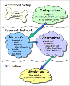1.1 ResSim Modules

ResSim offers three separate sets of functions called Modules that provide access to specific types of data within a watershed. These modules are Watershed

Setup, Reservoir

Network, and Simulation. Each module has a unique purpose and an associated set of functions accessible through menus, toolbars, and schematic elements. Figure 1.1 illustrates the basic modeling features available in each module. Figure 1.1. HEC-ResSim Module Concepts

1-1

1.1.1 Watershed Setup Module

The purpose of the Watershed Setup module is to provide a common framework for watershed creation and definition among different modeling applications. This module is currently common to HECResSim, HEC-FIA, and the CWMS CAVI.

A watershed is associated with a geographic region for which multiple models and area coverages can be configured. A watershed may include all of the streams, projects (e.g., reservoirs, levees), gage locations, impact areas, time-series locations, and hydrologic and hydraulic data for a specific area. All of these details together, once configured, form a watershed framework.

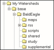When you create a new watershed,

ResSim generates a directory structure (see figure at right) for all files associated with the watershed.

In the Watershed Setup module, you assemble items that describe a watershed's physical arrangement. Once you have created a new watershed, you are able to import maps from external sources, specify the units of measure for viewing the watershed, add layers containing additional information about the watershed, create a common stream alignment, and configure elements. You can also add projects and create time-series icons within the Watershed Setup module.

Chapters 3 through 7 describe the Watershed Setup module in more detail.

1.1.2 Reservoir Network Module

The purpose of the Reservoir Network module is to isolate the development of the reservoir model from the output analysis. In the Reservoir Network module, you will build your network schematic, describe the physical and operational elements of your reservoir model, and develop the alternatives that you want to analyze. Using configurations that are created in the Watershed Setup module as a template, you will create the basis of a reservoir network. You will then add routing reaches and possibly other network elements to complete the connectivity of your network schematic. Once the schematic is complete, physical and operational data for each network element are defined. Also, alternatives are created that

1-2

specify the reservoir network, operation set(s), initial conditions, and assignment of DSS pathnames (time-series mapping).

Chapters 8 through 13 describe the Reservoir Network module in more detail.

1.1.3 Simulation Module

The purpose of the Simulation module is to isolate output analysis from the model development process. Once the reservoir model is complete and the alternatives have been defined, the Simulation module is used to configure the simulation. The computations are performed and results are viewed within the Simulation module.

When you create a simulation you must specify a simulation time window, a computation interval, and the alternatives to be analyzed. Then, ResSim creates a directory structure within the rss folder of the watershed that represents the simulation. Within this simulation tree will be a copy of the watershed, including only those files needed by the selected alternatives. Also created in the simulation is a DSS file named simulation.dss, which will ultimately contain all the DSS records that represent the input and output for the selected alternatives. Additionally, elements can be edited and saved for subsequent simulations.

Chapter 14 describes the Simulation module in more detail.

1.2 About this Manual

This User's Manual is the primary reference for providing ResSim users with detailed instructions for creating ResSim models and analyzing simulation results. With the exception of the first and second chapters, (which deal with introductory and core concepts), the chapters of this manual group tasks according to module. Each chapter provides an overview of key concepts and a detailed description of screen components and tools available in the module, and then shows you how to carry out specific tasks in the module. Appendices cover topics and tasks that require levels of detail beyond the scope of an individual chapter.

The organization of this manual is summarized in Table 1.1.

The HEC-ResSim Quick Start Guide is a separate document that provides a brief introduction and overview of the HEC-ResSim capabilities and includes references to this User's Manual for detailed information.

1-3

Table 1.1 Summary of Contents of HEC-ResSim User's Manual

HEC-ResSim Module	If you want to find out…	Refer to…
	Concepts of HEC-ResSim	Chapter 2
	How to create and manage watersheds	Chapter 3
	How to work with map layers	Chapter 4
	How to establish a stream alignment	Chapter 5
Watershed Setup Reservoir Network Simulation	How to create and define watershed elements and projects (e.g., reservoirs, levees, etc.) How to create computation points (hydrograph locations) How to create watershed configurations How to develop reservoir networks How to edit element data (junctions, routing reaches and diversions) How to define physical reservoir data How to edit physical reservoir data How to develop reservoir operation data How to define reservoir systems How to define alternatives How to develop and execute simulations How to analyze results How to calibrate model How to manage simulations Detailed application settings How to define the coordinate system How to edit maps How to change colors How to use HEC-DSSVue How to copy, export, and print tables References	Chapter 6 Chapter 6 Chapter 7 Chapter 8 Chapter 9 Chapter 10 Chapter 10 Chapter 11 Chapter 12 Chapter 13 Chapter 14 Chapter 14 Chapter 14 Chapter 14 Appendix A Appendix B Appendix C Appendix D Appendix E Appendix F Appendix G

1-4

Chapter 2

ResSim Concepts

Table of Contents

Section Page

2 RESSIM CONCEPTS ............................................................................................. 2-1

2.1 STARTING RESSIM ..........................................................................................2 -2 2.2 RECOGNIZING COMMON SCREEN COMPONENTS................................................ 2-3

2.2.1 MENU BAR...........................................................................................2 -3 2.2.2 MODULE LIST .......................................................................................2 -5

2.3 WATERSHED SETUP MODULE ...........................................................................2 -6 2.4 RESERVOIR NETWORK MODULE ..................................................................... 2-10 2.5 SIMULATION MODULE..................................................................................... 2-13 2.6 OPENING AN EXISTING WATERSHED ............................................................... 2-15 2.7 UNDERSTANDING SCHEMATIC ELEMENTS ........................................................ 2-17

2.7.1 STREAM ALIGNMENT .......................................................................... 2-17 2.7.2 OTHER WATERSHED ELEMENTS ......................................................... 2-17 2.7.3 RESERVOIR NETWORK SCHEMATIC ..................................................... 2-19 2.7.4 USING SHORTCUT MENUS .................................................................. 2-20

2.8 PRINTING AND EXPORTING REPORTS .............................................................. 2-20

2.8.1 PRINTING REPORTS ........................................................................... 2-21 2.8.2 PRINT PREVIEW ................................................................................. 2-24 2.8.3 EXPORTING REPORTS TO A FILE ......................................................... 2-25

2-i

List of Figures

Figure
Number	Page
FIGURE 2.1	RESSIM INFORMATION SCREEN ..................................................................2 -2
FIGURE 2.2	RESSIM MAIN WINDOW ..............................................................................2 -2
FIGURE 2.3	FILE MENU ................................................................................................2 -4
FIGURE 2.4	VIEW MENU ...............................................................................................2 -4
FIGURE 2.5	TOOLS MENU ............................................................................................ 2-4
FIGURE 2.6	HELP MENU ...............................................................................................2 -5
FIGURE 2.7	WATERSHED SETUP MODULE .....................................................................2 -6
FIGURE 2.8	RESERVOIR NETWORK MODULE ............................................................... 2-10
FIGURE 2.9	SIMULATION MODULE ............................................................................... 2-15

FIGURE 2.10 TOOLS, OPTIONS DIALOG BOX, GENERAL TAB:

RELOAD LAST WATERSHED AT STARTUP ............................................... 2-16 FIGURE 2.11 OPEN WATERSHED DIALOG BOX ............................................................. 2-16 FIGURE 2.12 STREAM ALIGNMENT............................................................................... 2-17 FIGURE 2.13 RESERVOIR ............................................................................................ 2-18 FIGURE 2.14 LEVEE ...................................................................................................2 -18 FIGURE 2.15 DIVERSION .............................................................................................2 -18 FIGURE 2.16 CHANNEL MODIFICATION ........................................................................ 2-18 FIGURE 2.17 OFF-CHANNEL STORAGE ........................................................................ 2-18 FIGURE 2.18 OTHER PROJECT .................................................................................... 2-18 FIGURE 2.19 COMPUTATION POINTS ........................................................................... 2-19 FIGURE 2.20 IMPACT AREAS ....................................................................................... 2-19 FIGURE 2.21 TIME-SERIES ICONS ............................................................................... 2-19 FIGURE 2.22 RESERVOIR NETWORK SCHEMATIC ......................................................... 2-20 FIGURE 2.23 SELECTING A REPORT ............................................................................ 2-21 FIGURE 2.24 SELECT PRINT FROM REPORT'S FILE MENU ............................................. 2-21 FIGURE 2.25 SELECT PRINT FROM REPORT'S SHORTCUT MENU ................................... 2-22 FIGURE 2.26 PRINTING PROPERTIES, PAGE TAB .......................................................... 2-22

FIGURE 2.32 SELECT EXPORT FROM THE REPORT'S FILE MENU ................................... 2-25 FIGURE 2.33 SELECT EXPORT FROM REPORT'S SHORTCUT MENU ................................ 2-26

2-ii

Chapter 2

ResSim Concepts

Before you begin working with the individual modules available in ResSim, you will need to understand the concepts that will allow you to develop, access, and interact with watersheds in ResSim.

This chapter begins with the following basics: explaining how to start ResSim; describing screen components that are common across modules, including menu items and map/mouse tools; and showing you how to create a new watershed or open an existing watershed.

Next, you will learn about the following four kinds of schematic elements in ResSim: Time-Series Icons, the Stream Alignment, Watershed (Study) Components, and the Model Schematic. This chapter also explains how to interact with schematic elements using right-click shortcut menus, which allow you to plot and tabulate data, edit model data, and edit common components of the watershed.

Layers are another concept in ResSim. This chapter will help you to understand how layers work in ResSim and describe the six kinds of layers: Time Series, Study, Stream Alignment, Gridded Data, Model Schematic, and Maps.

To work with Layers, you will use the Layer Selector. This chapter describes the components of the Layer Selector, including its menu items and layout, and shows you how to control layer display using the Layer Selector. You will learn how to view layer legends, organize layers, configure toolbar icons to control layer display, and add and remove map layers.

Each layer has a unique set of properties that you can configure to make your watershed display look the way you prefer. This chapter shows you how to use Properties Editors and other tools to configure the properties of Time Series, Study, Stream Alignment, Gridded Data, Model Schematic, and Map layers.

2.1 Starting ResSim

To begin working with the Watershed Data Sets, you must first start ResSim. Either double-click the HEC-ResSim icon on your PC's desktop, or from the Start menu, select Programs → HEC → ResSim. Once you start ResSim, an information screen (as shown in Figure 2.1) will appear briefly; then, ResSim's Main Window will open (Figure 2.2).

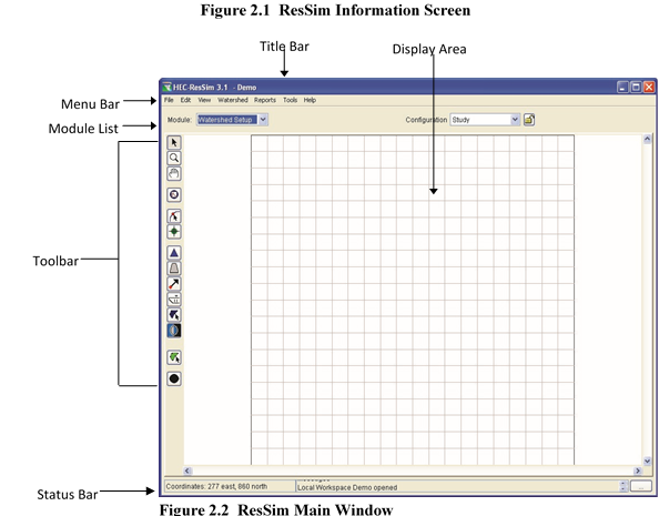
2.2 Recognizing Common Screen Components

ResSim offers three modules, each with its own functions and modulespecific tools, menus, and output. However, the modules share common screen components, as previously illustrated in Figure 2.2.

The Title Bar displays the ResSim title. After a watershed is opened, the name of the watershed will appear.

The Menu Bar contains menus for the modules. The items on the menus change as you switch between the modules, offering module-specific commands. You can select a menu item by clicking on the name of the menu (such as File), then pointing and clicking on the item you wish to select. Section 2.2.1 describes the Menu Bar in more detail.

The Module List contains all the available modules of ResSim. Use this list to move between the Watershed Setup module, the Reservoir Network module, and the Simulation module. Section 2.2.2 describes the Module List in more detail.

The Display Area is the geographic-referenced (geo-referenced) map space where all model schematic objects (reservoirs, junctions, diversions, etc.), watershed objects (stream alignments, reservoirs, stream reaches, etc.), and map layers are shown. You can manipulate elements and view results in the modules through the use of the tools in the Toolbar. Tools that affect the Display Area can have different functions depending on which module is selected.

The Status Bar displays map coordinates of the pointer in the display area when you are interacting with the watershed. When the pointer is outside of the display area, the Status Bar reflects the status of the program.

The General Message Bar displays a scrolling list of messages. System output log information appears in this window from the time you start ResSim until you exit the program. The scroll buttons on the right end of the Message Bar control the display and allow you to review all messages received during your ResSim session.

2.2.1 Menu Bar

In the Menu Bar, the File, View, Tools, and Help menus contain commands you can access from all three ResSim modules. Some of these menus also contain module-specific commands that appear only within individual modules. Commands and options that are common to all three modules are described as follows:

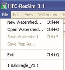The File menu (Figure 2.3) allows you to create a New Watershed, Open an existing watershed, Save a watershed, Save Map (the Display Area) and Exit ResSim. Your most-recently-used watersheds are located at the bottom of the File menu. When a watershed is opened, the remaining menu items become active.

Figure 2.3 File Menu

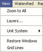In the View menu (Figure 2.4), select Zoom to All to restore your watershed view to full size after zooming in on one portion. Layers… opens the Layers Selector dialog box which is used to select the spatially referenced layers (map/coverage). Unit System allows you to see the current screen view settings. You can view data using

whichever Unit System you prefer (English Figure 2.4 View Menu

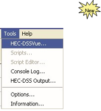or SI); however, the Watershed (native) Unit System is established when a watershed is created (see Chapter 3, Section 3.3.3) and cannot be changed afterward (see Tools menu for Watershed information). If a dialog or editor window is open but inactive, Restore Windows brings the dialog or editor window to the front as the active window. The Grid Lines option allows for turning on or off the grid lines in the map region.

The Tools menu (Figure 2.5) provides access to HEC-DSSVue, which you will use to view (and possibly edit) dssfiles that are used for storing primarily timeseries data. The Scripts and Scripts Editor commands allow you to create, open and edit scripts (the scheduling of scripts is accomplished in the Simulation

Module, from the Edit Menu). The

Console Log displays messages written to ^{Figure 2.5 Tools Menu}the "HEC-ResSim.log" file (typically found in the User's Documents and Settings folder named "…logs", e.g., "C:Documents and SettingsusernameApplication Data HECHEC-ResSim3.1logs") and contains information produced during the current program execution of ResSim. The HEC-DSS Output is a temporary log file that contains messages produced when dssfiles are accessed.

Options… provides for the following specifications: Model Directories (watershed locations for storing your watersheds); Compute Display settings (set the colors for compute messages and the format of log files); Debug Levels (set the level of debug messages); General (choose whether or not you want a confirmation message to appear when you exit ResSim and choose whether you want the last watershed reloaded at startup of the program); and, Fonts (for various window components).

Information… provides details about client, user, and watershed settings as well as server and system properties.

In the Help menu (Figure 2.6), the About HEC-ResSim command

displays information about the version of ResSim. Also, from this menu you can access user documentation and Install Example Watersheds (after

you define a watershed location as

described in Section 3.3.1). Figure 2.6 Help Menu

In addition to the four common menus described above, the following two menus appear in all three modules but contain module specific commands:

Edit – Typically, the edit options will be relevant to data element(s) for a specific module. The edit options available for each module are described in more detail in subsequent sections of this chapter.

Reports – Provides access to reports produced for a specific module. The reports available for each module are described in more detail in subsequent sections of this chapter.

2.2.2 Module List

From the ResSim main window (Figure 2.2) the graphical user interface (GUI) is organized to provide the necessary information to enter data, review data, edit data, run a simulation, and view results. The steps are divided into separate sets of functions called modules. A module has a specific set of commands that are accessed through menus and toolbars. Each module provides access to specific types of data or results. The modules of ResSim are as follows:

Watershed Setup – create a stream alignment, define projects (e.g., reservoirs, levees), define computation points, identify impact areas, create configurations for the watershed, and define time-series icons that represent specific locations or time-series identifiers. Section 2.3 provides more details of this module.

Reservoir Network – create networks, add routing reaches, edit elements, create and edit alternatives including assigning the DSS pathnames for time-series references. Section 2.4 provides more details of this module.

Simulation – define simulations for a watershed. A simulation consists of a time window and the ResSim alternatives you wish to execute for the simulation. Within this module, you can also edit element data. Once a simulation is defined, a compute is performed and the results are analyzed using graphical and tabular output. Section 2.5 provides more details of this module.

Each module has a menu bar and toolbar that are very similar for all of the modules. Example windows for each of the modules are presented in subsequent sections of this chapter.

2.3 Watershed Setup Module

The Watershed Setup module is used to create and setup your watershed. From the Module list, select Watershed Setup. The main window and the different components for the Watershed Setup module are illustrated in Figure 2.7.

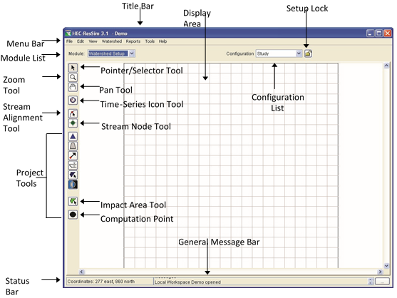
Figure 2.7 Watershed Setup Module

The Menu Bar (in Figure 2.7) contains the menus for the Watershed

Setup module. In addition to the four common menus described in Section 2.2.1, the following list is a description of the available menus in the Watershed Setup module.

Edit – From this menu, you can edit study information and view watershed information, edit global information for impact areas and projects, and adjust the colors and fonts used by the individual projects. Also, you can set the lock for editing the stream alignment and/or configurations. Available commands are:

Watershed Data, All Impact Areas, Projects, Drawing Properties, and Allow Editing.

Watershed – From this menu, you will create and edit configurations. You can also import and/or export the Stream Alignment and Impact Areas. Available commands are: Configuration Editor, Update Computation Points, Import, Export, and Save Configuration.

Reports – From this menu, you can review reports. These reports contain information about the streams, watershed elements, and configurations for the watershed. The available reports are: List of Streams, List of Impact Areas, List of All Configurations, List of Computation Points, and Projects.

The Configuration List (in Figure 2.7) shows the current configuration. Configurations are created, edited, and deleted in the Watershed Setup module. See Chapter 7 for discussion on Watershed Configurations.

The Setup Lock (in Figure 2.7) allows you to edit the stream alignment and the current configuration. This lock prevents others from editing the stream alignment and configuration elements while you are editing (i.e., "lock" others out so you can make changes).

The Display Area (in Figure 2.7) is where you create and view the stream alignment, projects, impact areas, and computation points through the use of the available tools in the Watershed Setup module. The following are descriptions of the available tools:

Pointer/Selector Tool –this tool can be used to edit, rename, and delete elements. To access, select the Pointer/Selector Tool, click the right mouse button (right-click) on an element, and the commands are available from a shortcut menu.

Zoom Tool - this tool allows zooming in and out of the display area. To zoom in, hold the left mouse button down and outline the area you want to zoom in on. To zoom out, right-click in the display area.

Pan Tool – this tool can be used to move the display area while you are zoomed in. To do this, hold down the left mouse button and drag the mouse in the direction you would like to pull the display area.

Time-Series Icon Tool - this tool is used to create, delete, and rename time-series icons used for plotting and tabulating timeseries data. To create, select the Time-Series Icon Tool, hold down the CTRL key and click. To access the available commands, select the Time-Series Icon Tool, right-click on a time-series icon, and the commands are available from the shortcut menu.

Stream Alignment Tool - this tool is used to create, delete, and edit stream elements that make up the stream alignment.

Stream Node Tool - this tool is used to create, delete, and edit stream nodes on the stream alignment.

Impact Area Tool - this tool is used to create, delete, rename, and edit impact areas. To create, select the Impact Area Tool; hold down the CTRL key while clicking the mouse button. Each click creates a vertex point, which is the boundary of the polygon. When reaching the end point, release the CTRL key and doubleclick. An impact area element is now visible. To access the available commands, select the Impact Area Tool, right-click on the impact area, and the commands are available from the shortcut menu.

Computation Point Tool - this tool is used to create, edit, rename, and delete computation points. Computation points are locations where time-series information is to be exchanged between models. For ResSim, this might be a control location for reservoir operations, a location where flows will be input, a location where a hydrograph is needed for FIA, etc. To create a computation point, select the Computation Point Tool, hold down the CTRL key and click on the stream alignment at the appropriate location. To access the available commands, select the Computation Point Tool, right-click on the computation point, and the commands are available from the shortcut menu.

Project Tools:

Reservoir Tool - this tool is used to create, delete, and rename reservoirs and to edit reservoir setup data (e.g. Description, Label Position, Year in Service, etc), as described in Chapter 6, Section 6.1.1). To create a reservoir, select the Reservoir Tool. A reservoir has to be created on the stream alignment. Hold down the CTRL key and click on the upstream end of the reservoir pool, release the CTRL key, drag along the stream alignment to the downstream end of the reservoir pool and click, and then name the reservoir. To access available commands, select the Reservoir Tool, right-click on the reservoir, and the commands are available from the shortcut menu.

Levee Tool - this tool is used to create, delete, rename, and edit levees. To create a levee, select the Levee Tool. A levee has to be created on the stream alignment. Hold down the CTRL key and click on the upstream end of the levee, release the CTRL key, drag along the stream alignment to the downstream end of the levee and click. To access available commands, select the Levee Tool, rightclick on the levee, and the commands are available from the shortcut menu.

Diversion Tool - this tool is used to create, delete, rename, and edit diversions. To create a diversion, select the Diversion Tool. A diversion has to begin on the stream alignment. Hold down the CTRL key and click on the stream alignment. Each click creates a vertex point, along the diversion. When reaching the end point of the diversion release the CTRL key, and click. To access available commands, select the Diversion Tool, right-click on the diversion, and the commands are available from the shortcut menu.

Channel Modification Tool - this tool is used to create, delete, rename, and edit channel modifications. To create a channel modification, select the Channel Modification Tool. A channel modification has to be created on the stream alignment. Hold down the CTRL key and click on the upstream end of the channel modification, release the CTRL key, drag along the stream alignment to the downstream end of the channel modification and click. To access available commands, select the Channel Modification Tool, right-click on the channel modification, and the commands are available from the shortcut menu.

Off-Channel Storage Area Tool - this tool is used to create, delete, rename, and edit off-channel storage areas. To create an off-channel storage area, select the Off-Channel Storage Area Tool and hold down the CTRL key while clicking the mouse button. Each click creates a vertex point, which is the boundary of the polygon. When reaching the end point, release the CTRL key and double-click. An off-channel storage area element is now visible. To access available commands, select the Off-Channel Storage Area Tool, right-click on the off-channel storage area, and the commands are available from the shortcut menu.

Other Project Tool - this tool is used to create, delete, rename, and edit other projects. This tool enables the placement of elements that represent "other" projects, such as pump stations and gages. To create an "other" project, select the Other Project Tool and hold down the CTRL key and click. To access available commands, select the Other Project Tool, right-click on the other project, and the commands are available from the shortcut menu.

2.4 Reservoir Network Module

The Reservoir Network module is used for editing element data and placing additional elements onto the stream alignment. From the Module list, select Reservoir Network. The main window and the different components for the Reservoir Network module are illustrated in Figure 2.8.

Figure 2.8 Reservoir Network Module

Your network elements will not be shown in the Display Area until you create or open a network from the Network Menu.

The Menu Bar (in Figure 2.8) contains the menus for the Reservoir Network module. After a reservoir network has been created or opened and is shown in the Display Area, the menus and their commands will become active. In addition to the four common menus described in Section 2.2.1, the following list is a description of the available menus in the Reservoir Network module.

Edit – From this menu, you can edit Reservoirs, Routing Reaches, Junctions, Diversions, and Reservoir Systems. State Variables can be created or edited, and Elements can be Imported. Also, you can set the lock for editing the reservoir network. Available commands are: Reservoirs, Reaches, Junctions, Diversions, Reservoir Systems, State Variables, Import Elements, and Allow Network Editing.

Network – From this menu, you will create, open, save, rename and delete reservoir networks. You can also update a network to recognize revisions made to its configuration within the Watershed Setup module. Available commands are: New, Open, Edit, Save, Save As, Rename, Update Network from Configuration, Import Network, and Delete Networks.

Alternative – From this menu, you will open the Alternative Editor that will enable you to create, edit, save and delete alternatives. The only command available from this menu is Edit.

Reports – From this menu, you can review reports that list the elements for the currently opened network. These reports contain information about the reservoirs, routing reaches, junctions and diversions. Also, advanced network summary listings are available. The available reports are: Reservoir List, Reach List, Junction List, Diversion List, and Advanced.

The Network box (in Figure 2.8) shows the "currently opened" Reservoir Network. You will not see a watershed schematic in the Display Area until you create or open a network.

The Configuration box (in Figure 2.8) shows the configuration the currently opened Reservoir Network is based upon. If you make changes to the network's Configuration (within the Watershed Setup module), then you can update the network(s) that use that configuration to recognize those revisions by selecting the Update Network from Configuration command from the Network menu.

The Network Lock (in Figure 2.8) allows you to edit the elements within the Reservoir Network. This lock prevents others from editing the elements while you are editing.

The Display Area (in Figure 2.8) is where you create the routing reaches for your Reservoir Network. Also, you can edit the elements through the use of the available tools in the Reservoir Network module. The following are descriptions of the available tools:

Pointer/Selector Tool –this tool can be used to edit, rename, and delete elements. To access, select the Pointer/Selector Tool, right-click on an element, and the commands are available from a shortcut menu.

Pan Tool –this tool can be used to move the display area while you are zoomed in. To do this, hold down the left mouse button and drag the mouse in the direction you would like to pull the display area.

Reservoir Tool – even though this tool can be used to create and delete reservoirs (which would normally be done within the Watershed Setup module) the typical use of this tool in the Reservoir Network module is for editing reservoir model data. Editing Physical and Operational reservoir data is discussed in detail in Chapter 10. To access available commands, select the Reservoir Tool, right-click on the reservoir, and the commands are available from the shortcut menu.

Diverted Outlet Tool - this tool is used to create, edit, rename, and delete diverted outlets from a reservoir. To create a diverted outlet, select the Diverted Outlet Tool. A diverted outlet must originate from a reservoir. Hold down the CTRL key and click on the appropriate reservoir, release the CTRL key, move the mouse pointer to a location in the watershed that will receive the diversion from the outlet and click. It is possible to create a diverted outlet that re-enters the network system. To do this, continue holding down the CTRL key and click to create vertex points and release the key when you are ready to place the final point back into the system. To access available commands, select the Diverted Outlet Tool, right-click on the diverted outlet, and the commands are available from the shortcut menu.

Routing Reach Tool - this tool is used to create, edit, rename, and delete routing reaches. A routing reach must be created between junctions and will follow the stream alignment. Attempting to create a reach where junctions don't exist will automatically generate junctions at the upstream and downstream ends of the reach. To create a routing reach, select the Reach Tool, hold down the CTRL key and click on the junction at the upstream end of the reach, release the CTRL key, drag along the stream alignment to the junction at the downstream end of the reach and click. To access available commands, select the Reach Tool, right-click on the routing reach, and the commands are available from the shortcut menu.

Junction Tool - this tool is used to create, edit and delete junctions. To add junctions (before creating routing reaches), select the Junction Tool, hold down the CTRL key and click on the stream alignment where you want to create the junction. To access available commands, select the Junction Tool, right-click on the junction, and the commands are available from the shortcut menu.

Diversion Tool - this tool is used to create, edit, rename, and delete diversions. To create a diversion, select the Diversion Tool. A diversion must begin from a junction. Hold down the CTRL key and click on the junction from which the diversion will occur. If you continue to hold down the CTRL key, each click creates a vertex point along the diversion. When reaching the end point of the diversion release the CTRL key, and click. Diversions can reenter the network or leave the network system entirely. To access available commands, select the Diversion Tool, right-click on the diversion, and the commands are available from the shortcut menu.

2.5 Simulation Module

The Simulation module is used to perform a simulation (compute), edit element data and view results. From the Module list, select Simulation. The main window and the different components for the Simulation module are illustrated in Figure 2.9.

The Menu Bar (in Figure 2.9) contains the menus for the Simulation Module. After a simulation has been created or opened and is shown in the Display Area, the menus and their commands will become active. In addition to the four common menus described in Section 2.2.1, the following list describes the available menus in the Simulation Module.

Edit – From this menu, you can edit the list of scheduled Scripts, make an Alternative Active, and edit Reservoirs, Routing Reaches, Junctions, Diversions, Reservoir Systems, and State Variables.

Available commands are: Script List, Set Active Alternative, Reservoirs, Reaches, Junctions, Diversions, Reservoir Systems, and State Variables. Also available is the Run editor for the active alternative.

Simulation – From this menu, you can create, open, re-open, close, edit, save, and delete simulations. You can also get information about the currently opened simulation and define release and target elevation overrides. Available commands are: New, Open, Re-Open, Close, Simulation List, Replace from Base, Edit, Save, Delete, Info, Run Manager, and Release Overrides.

Alternative – From this menu, you can edit alternatives. This menu only becomes active when a simulation is open. The only available command is Edit.

Reports – The available reports summarize results and provide network input summaries for the currently opened simulation. Available commands are: Reservoir Summary, Flow Summary, Power Summary, Gates Summary, Stage Summary, Release Decision, User Reports, Compute, and Network.

The Display Area (Figure 2.9) is where your stream alignment and watershed elements are displayed. You can view simulation results and edit projects and computation points through the use of the available tools in the Simulation Module. The following are descriptions of the available tools:

Pointer/Selector Tool –this tool can be used to edit projects and computation points, plot hydrographs, and view results. To access this tool, select the Pointer/Selector Tool, right-click on a location and select commands from the shortcut menu.

Zoom Tool - this tool allows zooming in and out of the display area. To zoom in, hold the left mouse button down and outline the area to which you want to zoom. To zoom out, right-click in the display area.

The Control Panel (Figure 2.9) shows the time window for the currently selected simulation in the Simulation Module. Also from the Control Panel you can manipulate simulations and alternatives.

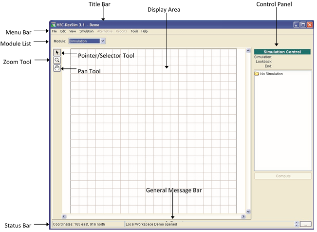
Figure 2.9 Simulation Module

2.6 Opening an Existing Watershed

With the ResSim main window open, you will need to open a watershed. In ResSim, a watershed is a data set associated with a geographic region for which you may configure multiple models and area coverages. A watershed may include all of the streams, projects (reservoir, levees), gage locations, impact areas, time-series locations, and hydrologic and hydraulic data for a specific area. All of these details together, once configured, form a watershed data set.

You may open an existing watershed from any of the modules (if you need to create a new watershed, refer to Chapter 3). Three methods of opening an existing watershed are available:

First, you can specify that your previously opened watershed be automatically opened by selecting Reload last Watershed at Startup from the General tab of the Options dialog box (Figure 2.10) from the Tools menu.

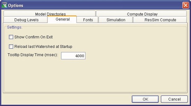
Figure 2.10 Tools, Options Dialog Box, General Tab: Reload last Watershed at Startup

Second, if you have opened the watershed before, you can select it from the list of most-recently-used watersheds, located at the bottom of the File menu.

Third, you may use the Open Watershed dialog to open the watershed, as follows:

On the File menu, click Open Watershed. The Open Watershed dialog box (Figure 2.11) will open.
Select a watershed from Available Watersheds (see
Chapter 3, Section 3.3.1 for
information on
defining Watershed

Locations). The Figure 2.11 Open Watershed Dialog Box

Current

Watershed box displays the watershed that is currently open, if any.

Click OK. The Open Watershed dialog box will close and the watershed you have selected will load and appear in the main window with the watershed name shown in the title bar.

You can have only one watershed open at a time. Therefore, if a watershed is open and you attempt to open another, the program prompts you to save the current watershed. If you do not save, any changes you have made to the current watershed will be lost.

2.7 Understanding Schematic Elements

Schematic elements in ResSim allow you to represent watershed, reservoir network, and simulation data visually in a geo-referenced context. You create schematic elements and edit their properties in the Watershed Setup Module (Chapters 3 through 7) and the Reservoir Network Module (Chapters 8 through 13). In the Simulation Module (Chapter 14), you can plot and tabulate data by using the shortcut menus associated with the schematic elements.

Stream Alignment
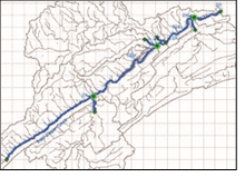The Stream Alignment (Figure 2.12) is a common component of the watershed. To create it, use the map (mouse) tools in the Watershed Setup Module to draw multi-segmented lines into the map display and to mark nodes and stream junctions.
Stream elements (segments), Figure 2.12 Stream Alignment stream nodes, and stream junctions are the components of a Stream Alignment. See Chapter 5 for more detailed information on creating and editing a Stream Alignment.
Other Watershed Elements
Other watershed elements include Projects, Computation Points, Impact Areas and Time-Series Icons. Create watershed elements in the Watershed Setup Module (Chapter 6).
These watershed elements are common components of a watershed that multiple models can reference (e.g., ResSim and FIA). To represent the elements, you use the Watershed Setup Module's map (mouse) tools to insert icons and draw polygons and multi-segmented

lines into the map display.

Projects include Reservoirs (Figure

2.13), Levees (Figure 2.14), Diversions

(Figure 2.15), Channel Modifications (Figure 2.16), Off-Channel Storage (Figure 2.17), and Other Projects like pump stations and agricultural diversions (Figure 2.18).

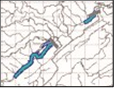
Figure 2.13 Reservoir

Figure 2.14 Levee

Figure 2.15 Diversion

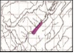
Figure 2.16 Channel

Modification

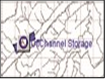
Figure 2.17 Off- Channel Storage

Figure 2.18 Other Project

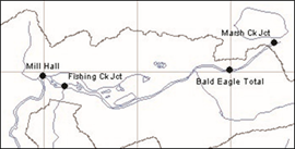Computation Points (Figure 2.19) are common points where data is exchanged between models (e.g., between ResSim and HEC-FIA). To represent these points, you use the

map (mouse) tools to insert

^{icons into the map display.}Figure 2.19 Computation Points

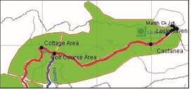Impact Areas (Figure 2.20) are common elements representing distinct portions of a watershed affected by rising stage in a stream, river, lake, or reservoir where flood damages will be evaluated.

Impact areas can be Figure 2.20 Impact Areas included in your ResSim model for consistency with your HEC-FIA model; however, the only computations performed in ResSim are related to the computation points corresponding to the FIA index locations.

For more information about Impact Areas, refer to the HEC-FIA User's Manual (HEC, 2003).

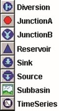Time-Series Icons (Figure 2.21) indicate sites where time-series data is available. You can use Time-Series Icons to represent the locations of gages or Time-Series locations.

For more information about Time-Series Icons, refer to the CWMS User's Manual (HEC, 2010).

Figure 2.21

Time-Series Icons

2.7.3 Reservoir Network Schematic

The Reservoir Network Schematic, which you develop in the Reservoir Network Module (based on a Configuration created in the Watershed Setup module), is a template for simulation computations. The graphical elements allow you to access data editors and specify properties of reservoir network components.

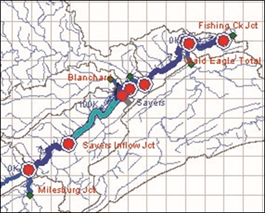The Reservoir Network Schematic (Figure 2.22) displays geo-referenced^*, graphical representations of Reaches, Diversions, Junctions, and

Reservoirs. When you interact with these representations in the Simulation Module, you

are able to view results

from the ResSim model's

observed and computed Figure 2.22 Reservoir Network Schematic hydrographs.

Geo-referencing does not influence ResSim's model data (i.e., Routing criteria is not automatically changed if adjustments are made to the Stream Alignment).

The Schematic is visible in the Reservoir Network module only when a Network has been opened and in the Simulation module only when a Simulation Alternative is set as active.

2.7.4 Using Shortcut Menus

Shortcut menus display when you right-click on schematic elements in the map display and other ResSim components such as plots, tables, and "tree structures". In ResSim, shortcut menus offer a variety of commands and options that allow you to access data editors, plot and tabulate data, view reports, compute Simulations, and more. Specific shortcut menu commands and options are described throughout this manual.

2.8 Printing and Exporting Reports

From each individual report there is a shortcut menu that allows you to print the report, preview the report before you print, and export the report to an ASCII delimited file. Right-clicking on the active report accesses the shortcut menu. Another way to print or export the reports is by clicking on Export or Print from the report's Report menu (in the Reservoir Network or Simulation module) or from the report's File menu (in the Watershed Setup module). Either method accesses the same dialog boxes.

2.8.1 Printing Reports

The output will be a print of the screen image of the active report. If items in the columns of the report are not printing, you can use the mouse to resize the column widths and the width of the entire report dialog box if you need to see more detail. To do so, roll the mouse pointer over one of the lines that delimit the columns or over the dialog box border. You can click on that line with the left mouse button and drag the mouse from side to side to indicate how wide you want the columns or dialog box. If you end up highlighting some cells in the table, then you probably moved the mouse slightly just before you pressed the button.

To print a report from the Watershed Setup module:

You must have a report selected (opened). For example, from the Reports menu in the Watershed Setup
module, select List of Computation Points (Figure 2.23).

From the File menu of the opened report, select Print (Figure 2.24). Or, you can right-click anywhere within the tabulated data of the report and from the shortcut menu select Print (Figure 2.25).

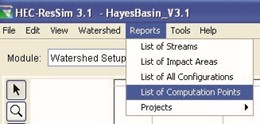
Figure 2.23 Selecting a Report

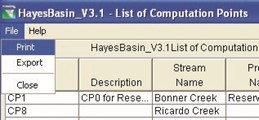
Figure 2.24 Select Print from

Report's File Menu

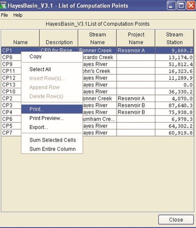
Figure 2.25 Select Print from Report's Shortcut Menu 3. The Print Properties dialog box will open (Figure 2.26).

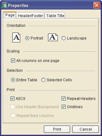
Figure 2.26 Printing Properties, Page Tab

From the Page tab (Figure 2.26), you can set the orientation (default is Portrait), make the report columns fit on one page, print the entire table (default) or print selected cells, repeat headers on subsequent pages, and display gridlines. By default the report prints in an ASCII format, if you want a screen image of the report, unclick ASCII and the report will print with any shading that you see on the report.
The Header/Footer tab (Figure 2.27) allows you enter a header and/or footer for the report.
The Table Title tab (Figure 2.28) allows you to change the default title of the report, and to determine whether you want the report title repeated on subsequent pages.

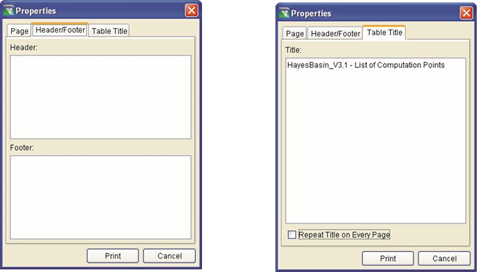
Figure 2.27 Printing

Properties, Header/Footer Tab

Figure 2.28 Printing

Properties, Table Title Tab

After you have everything set, click Print and the default system Print dialog box will open (Figure 2.29). Select the printer, and any other options you wish to set, click OK. The report will then be printed on the selected printer.

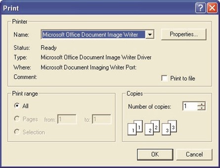
Figure 2.29 System Print Dialog Box

2.8.2 Print Preview

You can also preview the report before printing. To do so, do the following:

You must have a report selected (opened).
Right-click anywhere within the tabulated data of the report and from the shortcut menu, select Print Preview (Figure 2.30).

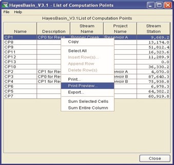
Figure 2.30 Select Print Preview from

Report's Shortcut Menu

The Properties dialog box (Figure 2.26) will appear.
Make the same adjustments for printing as described in Section
2.8.1. When you are satisfied, select Print from the Properties dialog box, and the Print Preview dialog box (Figure 2.31) will open.

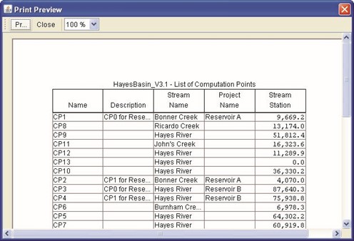
Figure 2.31 Print Preview Dialog Box

5. If you like what you see in the Print Preview dialog box, you can print by clicking Print, which opens the system Print dialog box (Figure 2.29), or you can close the Print Preview dialog box by clicking Close.

2.8.3 Exporting Reports to a File

You can also export reports to an ASCII delimited file. To export a report from the Watershed Setup module, do the following:

You must have a report selected (opened).
From the File menu
of the opened
report, select Figure 2.32 Select Export from the Export (Figure Report's File Menu
1. 32). Or, you can right-click anywhere within the tabulated data of the report and from the shortcut menu select Export (Figure 2.33).
  
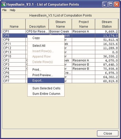
  Figure 2.33 Select Export from Report's Shortcut Menu

The Table Export Options dialog box (Figure 2.34) will open.
You can select the Field Delimiter from the list to be TAB,
SPACE, COMMA, SEMI-COLON, or COLON.
By default, the export does not use fixed width columns; however, if you want

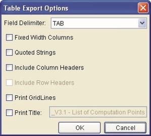
Figure 2.34 Table Export Options

Dialog Box

to do this you can click in the Fixed Width Columns checkbox.

You can also include the Quoted Strings, Column Headers of the report (default), include Gridlines, and include the Title of the report.

Once you have chosen your desired options, click OK and the System Save Browser (Figure 2.35) will open.

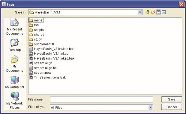
Figure 2.35 System Save Browser (for Saving a File)

You will need to select where you want the file to be saved and a filename. If you want the file to have an extension, you must enter your own; there is no default file extension.

Click Save and the System Save Browser will close. The filename that you entered will now be saved on your computer.

Chapter 3

Creating and Managing Watersheds

Table of Contents

Section Page

3 CREATING AND MANAGING WATERSHEDS ...................................................... 3-1

3.1 RECOGNIZING WATERSHED SETUP SCREEN COMPONENTS ................................ 3-1

3.1.1 MENU BAR...........................................................................................3 -2 3.1.2 CONFIGURATION SELECTOR AND LOCK/UNLOCK .................................... 3-4 3.1.3 MAP (MOUSE) TOOLS ...........................................................................3 -4

3.3.1 DEFINING A WATERSHED LOCATION ...................................................... 3-6 3.3.2 CREATING A NEW WATERSHED .............................................................3 -8 3.3.3 SPECIFYING UNITS OF MEASURE ..........................................................3 -9 3.3.4 SPECIFYING TIME ZONE........................................................................3 -9

3.4 SETTING UP NEW MAP LAYERS ........................................................................3 -9

3.4.1 IMPORTING MAPS INTO RESSIM ............................................................3 -9 3.4.2 ADDING A NEW MAP LAYER ................................................................ 3-12

3.4.3 SPECIFYING THE GEOGRAPHIC REFERENCING AND

COORDINATE SYSTEM ................................................................... 3-13

3-i

List of Tables

Table Page Number

TABLE 3.1 MAP LAYER FORMATS SUPPORTED BY RESSIM ........................................... 3-10

List of Figures

Figure Number

FIGURE 3.1 WATERSHED SETUP MODULE MAIN WINDOW .............................................. 3-2

FIGURE 3.2 FILE MENU ................................................................................................3 -3 FIGURE 3.3 EDIT MENU ................................................................................................3 -3 FIGURE 3.4 WATERSHED MENU ....................................................................................3 -3 FIGURE 3.5 REPORTS MENU ........................................................................................3 -3 FIGURE 3.6 RESERVOIR SHORTCUT MENU ....................................................................3 -6 FIGURE 3.8 ADD WATERSHED LOCATION DIALOG BOX ................................................... 3-7

FIGURE 3.9 CREATE NEW WATERSHED DIALOG BOX ..................................................... 3-8 FIGURE 3.10 LAYER SELECTOR DIALOG BOX ............................................................... 3-12 FIGURE 3.11 OPEN FILE DIALOG BOX TO ADD MAP LAYER ........................................... 3-12 FIGURE 3.12 GEOGRAPHIC REGION DIALOG BOX ......................................................... 3-13

3-ii

Chapter 3

Creating and Managing Watersheds

A watershed is a data set associated with a geographic region for which you may have configured multiple models and area coverages. A watershed may include all of the streams, projects (reservoir, levees, etc.), gage locations, impact areas, time-series locations, and hydrologic and hydraulic data for a specific area. All of these details together, once configured, form a watershed data set.

In the Watershed Setup Module, you will set up your watershed's physical arrangement including: background maps, the Stream Alignment, geo-extents, projects, and other geo-referenced data.

You define Configurations when you initially create a watershed. This should enable modelers to develop data explicitly for a specific configuration and reduce the possibility that incompatible model data sets will be used for multiple program applications (e.g., HEC-ResSim and HEC-FIA).

You can also use the Watershed Setup Module to define Projects and

Computation Points associated with specific configurations in your watershed.

Projects can include Reservoirs, Levees, Diversions, Channel Modifications, Off-Channel Storage Areas, and "Other" Projects. Computation Points are locations where time-series information is exchanged between models (e.g. ResSim and FIA).

3.1 Recognizing Watershed Setup Screen Components

The Watershed Setup Module provides tools for setting up your watershed's physical arrangement, including maps, the Stream Alignment, geo-extents, projects, and other geo-referenced data. Figure 3.1 shows the components of the Watershed Setup Module main window. Tools unique to this module are described in the following sections.

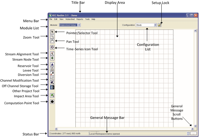
Figure 3.1 Watershed Setup Module Main Window

3.1.1 Menu Bar

The following is an overview of menus unique to the Watershed Setup Module. These tools will be described in more detail in the context of specific tasks later in this chapter.

Refer to Chapter 2 for information about the View, Tools, and Help menus, which are common to all three modules.

The File menu (Figure 3.2) allows you to create a New watershed, Open an existing watershed, Save a watershed, Save Map (saves the display area) and Exit ResSim. Your most-recently-used watersheds are located at the bottom of the File menu.

Use the Edit menu (Figure 3.3) to access the following editors in the Watershed Setup Module: the

Watershed Data Editor, All Impact Areas Editor, Projects Editor, and Drawing Properties Editor. You must select Allow Editing if you wish to make changes to your watershed (or toggle the Lock above the display area).

Using the Watershed menu

(Figure 3.4), you can create and edit

Configurations, Update

Computation Points, Import and

Export Stream Alignments, and Impact Areas, and Save Configurations.

The Reports menu (Figure 3.5) gives you access to reports for your watershed. Reports include the List of Streams, List of Impact Areas, List of All Configurations, List of Computation Points, and Projects listings by project type.

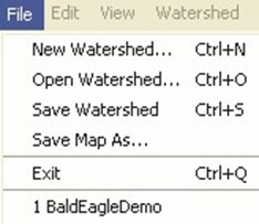
Figure 3.2 File Menu

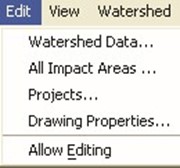
Figure 3.3 Edit Menu

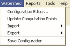
Figure 3.4 Watershed Menu

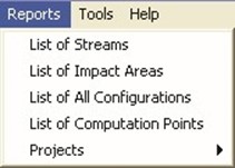
Figure 3.5 Reports Menu

3.1.2 Configuration Selector and Lock/Unlock

When you add a schematic element to the map display, you must choose its Configuration using the Configuration Selector. The default Configuration, Study, contains the entire set of all projects and Computation Points defined in the watershed. You can also associate projects with custom configurations.

Before you can add, remove, or edit schematic elements in your watershed, you must lock the Configuration by clicking on the symbol to the right of the Configuration Selector. When the Configuration is locked, the symbol appears. If the Configuration is unlocked, the symbol appears.

3.1.3 Map (Mouse) Tools

In the Watershed Setup Module, Map (Mouse) Tools allow you to access and configure objects within your watershed. Project Tools help you to create and edit the various project types. After you have created a project, ResSim adds it to the active Configuration. The following are descriptions of the available tools:

Pointer Tool

Right-click with the Pointer Tool to select and access a shortcut menu for any schematic element in the watershed map display.

Zoom Tool

Use the Zoom Tool to zoom in and out of the display area. To zoom in, hold the left mouse button down and outline the area you want to zoom in on. To zoom out, right-click in the display area.

Pan Tool

Use the Pan Tool to move the display area while you are zoomed in.

Time-Series Icon Tool

Use the Time-Series Icon tools to create, delete, and rename timeseries icons that are used for plotting and tabulating time-series data. To create, select the Time-Series Icon Tool, hold down the CTRL key and click. To access the available commands, select the TimeSeries Icon Tool, right-click on a time-series icon, and the commands are available from the shortcut menu.

Stream Alignment Tool

Use the Stream Alignment Tool to draw the multi-segmented lines that comprise a Stream Alignment representing river systems in the map display.

Stream Node Tool

The Stream Node Tool allows you to create and edit stream nodes and junctions, two of the primary components of a Stream Alignment.

Reservoir Tool

Use the Reservoir Tool to select and add reservoir projects to the map display and access editors for reservoirs.

Levee Tool

Use the Levee Tool to select and add levee projects to the map display panel and access editors for levees. In the Watershed Setup Module, only the name and description can be edited.

Diversion Tool

Use the Diversion Tool to select and add diversions to the map display and access editors for Diversions.

Channel Modification Tool

Use the Channel Modification Tool to select and add channel modifications (such as channel straightening, concrete walls, dredging, and widening) to the map display and access editors for Diversions.

Off Channel Storage Tool

Use the Off-Channel Storage Areas Tool to select and create OffChannel Storage Area polygons in the map display and edit their properties.

"Other" Project Tool

Use the "Other" Projects Tool to place icons representing "other" projects, such as pump stations and gages, etc., and edit their properties.

Impact Area Tool

Use the Impact Area Tool to create and edit impact areas representing regions in the watershed where flood damages will be evaluated.

Computation Point Tool

Use the Computation Point Tool to create and edit Computation Points. Computation Points are locations in the watershed where individual models will share information. Typically one model will produce results at a Computation Point that another model will use as input.

3.2 Using Shortcut Menus

Shortcut menu commands vary according to the schematic elements with which they are associated. Figure 3.6 shows the shortcut menu for a reservoir named "Reservoir A".

If your watershed is locked , the shortcut menu will allow you to edit, rename, delete the object (depending on the object type), remove from the activated

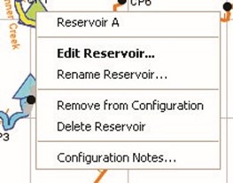
Figure 3.6 Reservoir Shortcut Menu

configuration, and add configuration notes, as well as import its properties. If your watershed is unlocked , some of the options will be unavailable.

3.3 Watershed Creation

The first thing you must do to create a new watershed is to specify its directory location, give it a name and description, and establish the Units of Measure and Time Zone. Once you have created your new watershed, ResSim generates a new directory hierarchy in the "base" working directory. Your new watershed becomes active in the main window and the tools needed to create the watershed data become available. At this point you may continue to configure the new watershed by adding layers and schematic elements, setting preferences for the map display, etc., as described later in this chapter.

3.3.1 Defining a Watershed Location

A Watershed Location is your working directory--the place on disk where you create and edit your watershed data. You can have multiple watershed locations, although an individual watershed cannot span multiple locations. Each watershed location should have a logical name, such as CWMS or General Projects.

Before you can create or open a watershed, you must define at least one watershed location. To define a Watershed Location:

From the Tools menu, select Options. The HEC-ResSim Options dialog box (Figure 3.7) will open.

Figure 3.7 HEC-ResSim Options Dialog Box

Select the Model Directories tab. The Name and Location of any watershed locations you have previously defined will display in the list.
To add a new location to the list, click the Add
Location…button. The Add Watershed Location dialog box will open (Figure 3.8).

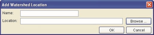
Figure 3.8 Add Watershed Location Dialog Box

Enter a logical Name for the new location, then click the Browse… button to select the area on disk where you want to build your watershed. This directory is the "holder" of the "base" directory and the "base" directory is the "holder" of your watershed. In other words, the Watershed Location contains a directory named base, which contains the directory(s) for your watershed(s).
Click OK to close the Add Watershed Location dialog box.

The new location will now appear in the list of watershed locations on the Model Directories tab.

Refer to Appendix A for information about other options available in the Options dialog box.

3.3.2 Creating a New Watershed

Once you have established the working directory, you can create a new watershed.

To create a new watershed:

Select New Watershed from the File menu. The Create New Watershed dialog box (Figure 3.9) opens.

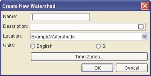
Figure 3.9 Create New Watershed Dialog Box

Type a Name for the new watershed. The watershed name must be less than 32 characters and cannot contain any of the following characters: | / : * ? " < > - .
Type a Description for the new watershed that clearly explains what it is.
Select a Location (working directory) for the new watershed's directory from your list of available locations.
Specify either English (U.S. customary units) or SI (System International) as the Units of Measure. You will not be able to change this after you click OK (see Section 3.3.3, Specifying Units of Measure, for more information).
Specify the Time Zone of the new watershed by selecting from the list of standard time zones. Note that the watershed Time Zone does not recognize Daylight Savings Time (see Section 3.3.4, Specifying Time Zone, for more information).
Click OK to close the Create New Watershed dialog box.

3.3.3 Specifying Units of Measure

All modeling data, time-series data, geometric and reservoir information, model parameters, and flow-, elevation- and stage-timeseries data must use the same unit system when saved. Therefore, it is crucial that you specify either English or SI as the Units of Measure for your watershed when you create it. NOTE: You cannot change the watershed units of measure once you have created the watershed. However, you can (at any time) customize the display of data using the View menu.

3.3.4 Specifying Time Zone

When a new watershed is created, the user must select the appropriate time zone for the watershed. This typically would be the time zone for the outlet or major portion of the watershed. Internally, ResSim will store all time-series data using the fixed "standard time offset from GMT" for the selected watershed time zone. Thus, internally, the data will be held in standard time only.

You cannot change the Watershed Units of Measure or the Time Zone once the watershed has been created.

3.4 Setting Up New Map Layers

Layers in ResSim are like transparencies laid one on top of the other, with static physical images such as roads, county and state boundaries, rivers, subbasins, etc., layered in the display as color pictures. Each of these images, along with its associated data, is a map layer. Access to the Layers Selector is available from the View menu. Refer to Chapter 4 for a more detailed description of Map Layers.

3.4.1 Importing Maps into ResSim

The background maps you will use in your watershed will come from sources outside of ResSim. To import a map file for use in your watershed, copy the appropriate map files to the "maps" directory of your watershed (see Appendix A for information about the ResSim directory structure). ResSim does not perform coordinate transformation for background maps. Therefore, all of the map layers you use in a watershed should be referenced to the same coordinate system (see Appendix B for more information on coordinate systems). Table 3.1 shows the file formats ResSim supports and each format is described in the paragraphs that follow. Appendix C describes how to access the map editors for configuring each type of map format.

Table 3.1 Map Layer Formats Supported by ResSim

Description	Common File Name Extension
ArcView® Shapefile	.shp
AutoCAD® DXF	.dxf
Raster image	.img, .gif, .jpg
USGS* Digital Line Graph	.dlg
USGS* Digital Elevation Model	.dem
ASCII NetTIN	.net
ArcInfo® DEM	.asc
*US Geological Survey

Arc Shapefiles (.shp)

This layer type is the native data structure for the ArcView® GIS program. Shapefiles store non-topological geometry and attribute information for the spatial features of a data set. Usually there are three files: *.dbf, *.shp, and *.shx. The .shp file contains the shapes (point, polylines, or polygons) that display in the layer. Each shape has a record in the .dbf file containing descriptive data called "attributes." The .shx file contains an index that links each shape to its record in the .dbf file.

AutoCAD® DXF (.dxf)

A Drawing Interchange file (.dxf) is created by a Computer-Aided Design (CAD) package, AutoCAD®. This format is a tagged data representation of an AutoCad® drawing file. In tagged data, a group code precedes each data element. A group code is an integer number indicating the type of data element. The file created is a vector-based graphic. The DXF format is commonly used for data exported from other CAD and GIS programs.

Raster Image

ResSim supports JPEG (.jpg) and Graphics Interchange (.gif) raster image formats. Before ResSim can access these file types, you must first create an .img (ASCII text) file containing the following lines:

Image West=2051443.

Image North=355443. These are image boundaries that are determined by the user and usually

Image East=2054925.6calculated using a program such as Image South=351947.4ArcInfo®.

Image URL = path and filename of raster image

(i.e., maps/lh_2m.gif)

The raster image boundaries must match the easting and northing parameters stated in the Geographic Region Dialog (see Section 3.4.3, "Specifying the Geographic Referencing and Coordinate System").

USGS Digital Line Graph (.dlg)

USGS Digital Line Graph (DLG) files are created from two sources using manual and automated digitizing methods. The two sources are aerial photographs and cartographic sources. DLG files are vector representations of the data. When ResSim interacts with a .dlg file, it automatically creates a .dlgbin file, which is a binary representation of the ASCII .dlg file.

USGS Digital Elevation Model (.dem)

The USGS Geological Survey publishes the raster file format USGS Digital Elevation Model (DEM). DEM files usually contain terrain elevations, but the file format can be used for representing any surface. The format, published by the USGS, allows internal documentation of coordinate system, date of publication, etc.

ASCII NetTin (.net)

This is an ASCII file format used to represent a Triangulated Irregular Network (TIN). The TIN data is stored in a simple format that defines the nodes, edges, and triangles contained in the TIN. This format is common for transferring TIN data between software packages.

ArcInfo® DEM (.asc)

This is an ASCII file format representation of a grid generated by ArcInfo®. The file consists of keywords followed by values defining the number of columns, number of rows, lower left corner, cell size, no data value, and each cell value.

3.4.2 Adding a New Map Layer

To make map files accessible in the watershed, first make sure that the map files are in the "maps" directory of the watershed, as previously described in Section 3.4.1. Also, ensure all maps you add to a watershed share the same coordinate system before you add them to the watershed.

To add a map layer to your watershed:

Select Layers from the View menu. The Layer Selector dialog box will appear (Figure 3.10).
From the Edit menu, select Allow Layer Editing.
Next, from the Maps menu, select Add Map

Layer. The Open File Figure 3.10 Layer Selector Dialog Box dialog box (Figure 3.11) will open.

Figure 3.11 Open File Dialog Box to Add Map Layer

Locate the map file you wish to use on your local computer (for example, "np_shed.shp").
After you have selected the map you wish to use, click OK. The new map will now appear in the Layer Selector dialog box.

3.4.3 Specifying the Geographic Referencing and

Coordinate System

To maintain a geographic reference, you must specify a coordinate system for each watershed. To establish the grid size and coordinate system:

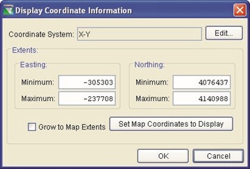Select Layers from the

View menu to open the Layer Selector dialog box.

From the Maps menu, select Map Display Coordinates to open the Geographic Region dialog box (Figure 3.12).

Figure 3.12 Geographic Region

Dialog Box

The Geographic Region dialog box includes the following information:

Coordinate System

This box identifies the coordinate system established for the watershed. The coordinate system can be edited, but remember that all maps and data must exist in one unified coordinate system. Therefore, some layers or data might require the use of a GIS program to transform coordinate system information. For additional information about editing the Coordinate System, see "Editing the Coordinate System" paragraph below.

Extents

The values of Easting Min, Easting Max, Northing Min, and Northing Max indicate the location of the left, right, bottom and top borders (respectively) of the grid in the display area. ResSim displays coordinates in the Status Bar as you move the cursor within the map display panel.

Grow to Map Extents

When you check this box, ResSim automatically sets the geographic region to define the smallest rectangle that encompasses all of the objects (maps, icons, alignments, etc.) in the display area. If you add any objects to the watershed that lie outside the geographic region,

ResSim automatically updates the extents to include the new objects.

You must select the geographic extents of your watershed carefully to ensure that all map layers in your watershed setup are included. The extents you specify and the coordinate system you use must be consistent for all layers in the watershed. You should use GIS tools to transform layers from one coordinate system to another before you use them in ResSim.

Setting Map Coordinates to Display

You can automatically set the geographic extents to the coordinates in your current view. First, zoom in or out in the display area to determine a preferred geographic region, then open the Geographic Region dialog box and click Set Map Coordinates to Display.

ResSim will set the extents to the current view in your map display. Objects beyond the geographic extents remain in the watershed, but they are not included in the grid of the display area.

Editing the Coordinate System

You can edit the Coordinate System of the Watershed by selecting

Edit in the Geographic Region dialog box. This opens the Map Coordinate Information dialog box, where you can configure the

System, Units, Spheroid, and other system-specific data. See Appendix B for more information on configuring map coordinate information.

Chapter 4

Working with Layers

Table of Contents

Section Page

4 WORKING WITH LAYERS .....................................................................................4 -1

4.1 UNDERSTANDING LAYERS ................................................................................4 -1

4.1.1 TIME-SERIES ICON LAYER ....................................................................4 -1 4.1.2 STUDY LAYER ......................................................................................4 -1 4.1.3 STREAM ALIGNMENT LAYER ..................................................................4 -2 4.1.4 MAP LAYERS .......................................................................................4 -2

4.2 EXPLORING THE LAYER SELECTOR ...................................................................4 -2

4.2.1 THE LAYER SELECTOR MENUS .............................................................4 -3 4.2.2 THE LAYER SELECTOR "TREE" ..............................................................4 -4 4.2.3 CONTROLLING LAYER DISPLAY .............................................................4 -5 4.2.4 VIEWING LAYER LEGEND ......................................................................4 -6

4.3 CONTROLLING LAYER ORGANIZATION ...............................................................4 -6

4.3.1 CONFIGURING TOOLBAR ICONS TO CONTROL LAYERS ............................ 4-7 4.3.2 ADDING MAP LAYERS ...........................................................................4 -8 4.3.3 REMOVING MAP LAYERS ......................................................................4 -8 4.3.4 USING LAYER SELECTOR SHORTCUT MENUS ......................................... 4-9

4.4 VIEWING AND CONFIGURING LAYER PROPERTIES ............................................ 4-10

4.4.1 STUDY LAYER PROPERTIES ................................................................ 4-11 4.4.2 STREAM ALIGNMENT LAYER PROPERTIES ............................................ 4-15 4.4.3 MAP LAYERS PROPERTIES .................................................................. 4-16

4-i

List of Figures

Figure Number	Page
FIGURE 4.1	LAYER SELECTOR ......................................................................................4 -2
FIGURE 4.2	LAYERS MENU - LAYER SELECTOR ..............................................................4 -3
FIGURE 4.3	EDIT MENU - LAYER SELECTOR ..................................................................4 -3
FIGURE 4.4	EDIT MENU - ALLOW LAYER EDITING TURNED OFF AND

NO LAYER SELECTED ...........................................................................4 -3

FIGURE 4.5	MAPS MENU - LAYER SELECTOR ................................................................. 4-4
FIGURE 4.6	VIEW MENU - LAYER SELECTOR ................................................................. 4-4
FIGURE 4.7	LAYER SELECTOR - LAYERS EXPANDED ...................................................... 4-5
FIGURE 4.8	LAYER SELECTOR - MAP LEGEND FOR RESERVOIRS .................................... 4-6
FIGURE 4.9	TOOLBAR BUTTON EDITOR .........................................................................4 -7

FIGURE 4.10 LAYER SELECTOR - SHORTCUT MENU FOR THE

STREAM ALIGNMENT LAYER ..................................................................4 -9

FIGURE 4.16 DRAWING PROPERTIES EDITOR - COMPUTATION POINT TAB ..................... 4-13 FIGURE 4.17 DRAWING PROPERTIES EDITOR - IMPACT AREA TAB ................................. 4-14 FIGURE 4.18 STREAM ALIGNMENT PROPERTIES EDITOR ............................................... 4-15

FIGURE 4.19 USGS DIGITAL LINE GRAPH EDITOR FOR

DIGITAL LINE GRAPH (DLG) MAP LAYER, PROPERTIES TAB ................. 4-16

FIGURE 4.20 USGS DIGITAL LINE GRAPH EDITOR FOR

DIGITAL LINE GRAPH (DLG) MAP LAYER, SCALE TAB........................... 4-16

4-ii

Chapter 4

Working with Layers

4.1 Understanding Layers

Layers are hierarchical. Primary (top level) layers include the TimeSeries Icon Layer and the Study Layer (available only in the Watershed Setup Module), the Stream Alignment Layer, and Map Layers. These primary layers can contain component layers. For example, the Stream Alignment Layer contains the Stream Nodes, Stream Segments, and Stream Junctions. The Study Layer contains layers for all Reservoirs and other Projects, Computation Points, and Impact Areas contained within the Study.

4.1.1 Time-Series Icon Layer

The Time-Series Icon Layer includes all of the time-series icons for your watershed, and it allows you to separate different types of data in your map display. For example, a gage may report stage and precipitation (and compute flow from stage). If you create time-series layers named "Stage," "Flow," and "Precipitation," you can then place each data set in the appropriate layer.

ResSim does not use Time-Series Icons for any program needs. Refer to the CWMS User's Manual (HEC, 2010) for additional details about Time-Series Icons.

4.1.2 Study Layer

The Study Layer appears in the Watershed Setup Module only. The Study layer is comprised of all of the projects, impact areas, and computation points contained in the watershed.

The Layer Selector displays Study as a primary layer in the Layer tree. When you click on the root handle for the Study branch, there is a layer for Computation Points, Diversions, Names (labels for the projects, computation points, and impact areas), Reservoirs, Channel Modifications, Levees, Off Channel Storage, Other Projects, and Impact Areas. ResSim creates a layer for each of these items even before you have defined any projects, computation points, or impact areas.

4.1.3 Stream Alignment Layer

The Stream Alignment Layer contains the Stream Alignment representing the river system in the watershed. The Stream Alignment layer includes three component layers: Stream Nodes, Streams Segments (also referred to as stream elements), and Stream Junctions. This layer is available in all ResSim Modules but is only available for editing within the Watershed Setup Module.

4.1.4 Map Layers

ResSim can display various types of maps and elements in the georeferenced map display area. These maps, displayed as map layers, are static physical images. Examples of map layers include roads, county and state boundaries, rivers, subbasins, etc. Some maps are static images, which display as color pictures in the display area. Map Layers are not interactive. Instead, you interact with data associated with schematic elements you place in your map display.

For a description of the map layer formats supported by ResSim, see "Importing Maps into ResSim" in Chapter 3, Section 3.4.1.

4.2 Exploring the Layer Selector

The Layer Selector is the main controller for the organization of the various layer types described above, including the Study Layer, Stream Alignment Layer, and Map Layers.

To access the Layer Selector from any module, from the View menu, select Layers….

The Layer Selector window, shown in Figure 4.1, opens as a separate frame that you can minimize to the Windows taskbar.

Figure 4.1 Layer Selector

4.2.1 The Layer Selector Menus

Menus in the Layer Selector offer a variety of tools to assist you in

managing layers.

The Layers menu (Figure 4.2) offers a Close command to close the Layer Selector.

The Edit menu (Figure 4.3) provides tools for rearranging layers, viewing and editing layer properties, and adding and reloading default toolbar buttons for access to individual layers.

To see all of the available commands in the Edit menu, you

must first select a layer and activate Allow Layer Editing. When editing is enabled, a checkbox appears next to the menu item as shown in Figure 4.3.

Figure 4.4 shows the Edit menu as it appears with Allow Layer Editing turned off and with no layer selected.

Also note that the current position of an individual layer will determine which commands are available in the Edit menu. When

a layer is already at the top, the Move to Top and Move Up options will be unavailable. Likewise, if a layer is at the

bottom, the Move Down and Move to Bottom options will not be available.

Figure 4.2 Layers Menu -

Layer Selector

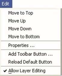
Figure 4.3 Edit Menu -

Layer Selector

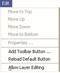
Figure 4.4 Edit Menu -

Allow Layer Editing Turned Off and No Layer Selected The Maps menu (Figure 4.5) allows you to add and remove map layers, as well as import images. The Map Display Coordinates option opens the Geographic Region dialog box. These processes are described in "Adding a New Map Layer" in Chapter 3, Section 3.4.2. You must select a map layer to access the Remove Map Layer command.

The View menu (Figure 4.6) gives you control over display of the Layer Selector. The Expand option expands the "tree" of a layer to display its sublayers (same functionality as clicking on the layer's plus- sign box in the tree). Once you have expanded a

Figure 4.5 Maps Menu -

Layer Selector

Figure 4.6 View Menu -

Layer Selector

layer, Expand changes to Collapse to close the layer to show only the primary layer (same functionality as clicking on the minus-sign box in the tree). Always on Top keeps the Layer Selector on top of your desktop so you can leave it open while you work, if desired.

4.2.2 The Layer Selector "Tree"

The Layer Selector uses a tree metaphor for controlling the display and organization of layers in the watershed. The tree metaphor represents the hierarchical arrangement of layers in ResSim.

The top level of the tree is the Layers folder, which contains all of the layers in the watershed. Beneath the Layers folder is a tree branch for each primary layer, beginning with a plus/minus box, followed by a checkbox, then the layer name.

When you expand a layer ("Controlling Layer Display" , Section 4.2.3), its sub-layers display. If no sub-layers exist, you will see a legend for the layer.

In following sections you will learn how to interact with layers in the Layer Selector by using the Menu items, shortcut menus, plus/minus boxes, checkboxes, and properties editors.

4.2.3 Controlling Layer Display

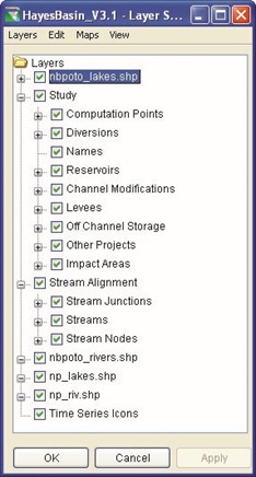Beside each Layer branch is a plus/minus box, or root handle, that serves the same function as the Expand/Collapse options in the View menu. A plus means the layer can be expanded. You can click on a plus to expand a tree branch to display component layers; if no component layers exist, you will see a legend for the layer. When the root handle is a minus, you can click on it to collapse the tree branch. You can also expand and collapse layers by double-clicking them with your mouse. Figure 4.7 shows the Layer Selector with some of the layers expanded.

The checkbox turns the display of

^{the layer on or off (checked}Figure 4.7 Layer Selector -

indicates the layer is active in the _{Layers Expanded} display area). When not checked, neither the primary layer nor the components beneath it will display. When checked, the primary layer and all checked component layers will display; however, any unchecked component layers beneath it will not display.

4.2.4 Viewing Layer Legend

When you click on the root handle of a layer with no components, the legend for the map displays.

The type of legend displayed is determined by the various file formats. Figure 4.8 shows the legend for Reservoirs.

Figure 4.8 Layer Selector -

Map Legend for Reservoirs

4.3 Controlling Layer Organization

The Layer Selector also controls how layers are arranged in the display area. When you add map layers to the watershed ("Adding a New Map Layer" in Chapter 3, Section 3.4.2), the map layer is added to the bottom of the list of maps in the Layer Selector. You can use the Layer Selector to rearrange the order of the primary layers:

Select the layer you would like to move.
From the Edit menu, select Allow Layer Editing.
From the Edit menu, select Move Up to move the layer towards the front of the map display, or click Move Down to move the layer to the back.
To see your changes, click Apply (to keep the Layer Selector open) or click OK to close the Layer Selector.

Continue to change the position of each layer until the necessary map features are visible in the display area.

4.3.1 Configuring Toolbar Icons to Control Layers

In the Layer Selector you can also add controls to the Toolbar of the main window. Toolbar buttons provide a shortcut for turning layers on and off without having to open the Layer Selector. Toggling on and off the toolbar button functions the same as the checkbox in the Layer Selector. When the button is depressed, the layer is selected for display in the map panel. When the button is up, the layer is turned off in the display. This shortcut is useful when you might want to have frequent control over layers that are being displayed.

Additionally, right-clicking on the toolbar button gives you access to various properties editors and allows you to select and deselect layers being displayed. The options available from the shortcut menu depend upon the layer type.

If you hover your mouse over a Toolbar Button, a Tool Tip appears with a description of the button.

Adding toolbar buttons is an optional configuration step, and if you want to use toolbar buttons, you must configure them separately in each module. Toolbar buttons are saved when you exit the watershed, so you will only have to set them up once.

To add a toolbar button:

In the Layer Selector, select a layer in the tree.
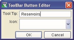From the Edit menu, select Add Toolbar Button. The Toolbar Button Editor opens, as shown in Figure 4.9.
The name of the layer appears by default in the Figure 4.9 Toolbar Button Tool Tip field, but you Editor can specify a more descriptive Tool Tip if desired.
From the Icon list, select an icon to represent the selected layer.
Select OK when you are done.

The toolbar button then appears in the toolbar above the Display Area.

To remove a toolbar icon, select the layer in the Layer Selector, and then from the Edit menu, select Remove Toolbar Button. To quickly remove all toolbar buttons that you have defined, select Reload Default Button from the Edit menu in the Layer Selector.

4.3.2 Adding Map Layers

You will find it helpful to add maps to the watershed and the display area to provide a geographical reference for time-series icons, the stream alignment, and projects in your watershed.

To add map layers:

From the Edit menu of the Layer Selector, select Allow Layer Editing.
From the Maps menu, select Add Map Layer… This command opens a file browser to the default "maps" directory in the watershed directory hierarchy. You must first copy any maps you wish to use in the watershed to the "maps" directory for your watershed.
From the file browser, choose the map you wish to add.
Click OK.

The map name now appears in the Layer Selector as a new tree branch. See "Adding a New Map Layer" in Chapter 3, Section 3.4.2 for more information.

4.3.3 Removing Map Layers

To remove a layer from the map display, select the layer in the layer selector, and then select Remove Map Layer from the Maps menu.

4.3.4 Using Layer Selector Shortcut Menus

Shortcut menus in the Layer Selector offer commonly used commands that are also available in the Layer Selector's Edit and View menus. Figure 4.10 shows the shortcut menu for the Stream Alignment layer in the Layer Selector.

The Expand option expands the tree of a layer to display its component layers. Collapse closes the layer to show only the primary layer.

Move to Top, Move Up,

Move Down, and Move to Bottom allow you to rearrange layers. The current position of an individual layer will

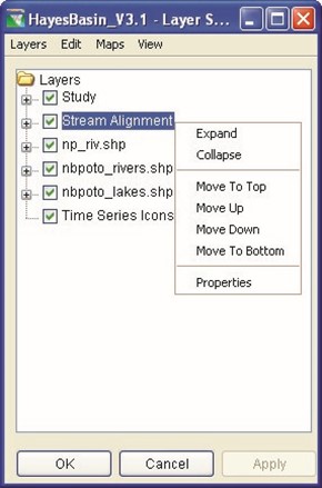
Figure 4.10 Layer Selector - Shortcut Menu for the

Stream Alignment Layer

determine which Move buttons are available.

Properties opens a Properties dialog box for the layer.

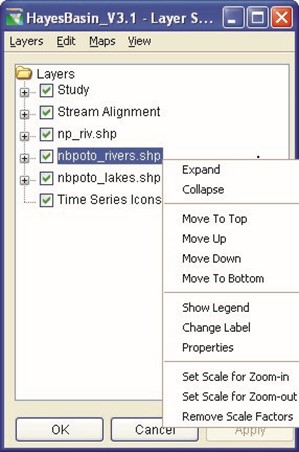For map layers that you add (Figure 4.11), there are several additional options available. The Show Legend option expands the map layer tree to display the map legend. This option changes to Hide Legend when the layer is expanded, allowing you to close the branch view of legends. Also, the Change Label option allows you to change the name of the layer in the tree.

The remaining options are related to when the layer should appear in the map

region. The viewing of the

layer can be made to depend

on the how "zoomed in" or "zoomed out" the view is in the map display area. These options include Set Scale for

Figure 4.11 Layer Selector -

Shortcut Menu for a

Map Layer

Zoom-in, Set Scale for Zoom-out, and Remove Scale Factors.

Reminder: you must first activate Allow Layer Editing (from the Edit menu) before you can access many of the shortcut menu commands.

4.4 Viewing and Configuring Layer Properties

The Layer Selector provides three ways to view and configure layer properties. You can:

Select a layer in the Layer Selector and then choose Properties from the Edit menu.
Right-click on a layer in the Layer Selector and then select Properties from the shortcut menu.
Double click on a layer in the Layer Selector.

Each of these techniques opens a Properties dialog box specific to the layer type; map layers also have additional dialog boxes for configuring properties. For information about configuring the Time-Series Icon Layer, refer to the CWMS User's Manual (HEC, 2010).

4.4.1 Study Layer Properties

The Study Layer is available only in the Watershed Setup module. When you select Properties for the Study layer, the Drawing Properties Editor appears (Figure 4.12).

The Drawing Properties Editor has six tabs that allow you to view and edit properties of Reservoirs, Levees, Diversions, Channel Modifications, Computation Points, and Impact Areas in your watershed.

Figure 4.12 Drawing Properties Editor - Reservoir Tab

With the Reservoir tab selected (Figure 4.12), you can choose the Fill and Outline Color for the Triangle (which is the "visual" representation of the Reservoir) and the Fill and Outline Color and the Width of the Storage Reach (which represents the Reservoir reach along the stream alignment) of reservoirs in your watershed display. Also, you can choose the Fill Color and Width of the Dam element. When you select Draw Reservoir Triangle with a checkmark, the reservoir shape drawn in the Watershed Setup Module displays on the map; when it is not checked, the reservoir shape does not display. Likewise, Draw Reservoir Name, when checked, displays the reservoir name on the map and hides the name when unchecked. The Font… button for the Reservoir Name allows you to choose the text font for the name of the reservoir in the map display.

The Levees tab (Figure 4.13) allows you to edit the properties of levees in your watershed. You can specify the Line Color and Levee Width. Draw Levee Name, when checked, displays Levee names on the map and hides the names when unchecked. The Font… button for the Levee Name allows you to choose the text font for the name of the levee in the map display.

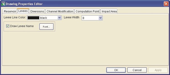
Figure 4.13 Drawing Properties Editor - Levees Tab

With the Diversions tab (Figure 4.14), you can select the Line Color and Width for the diversion. You can also select the Fill Color for the Diversion Arrowhead. The arrowhead colors can be different to indicate whether or not the diversion is Connected or Disconnected (e.g., Connected indicates that the diverted water remains in the system and Disconnected indicates that the diverted water is lost to the system). Draw Diversion Name, when checked, displays the Diversion names in the display area and does not display when the name is unchecked. The Name Font… button allows you to choose the text font for the name of the diversion in the watershed display area.

Figure 4.14 Drawing Properties Editor - Diversions Tab

The Channel Modification tab (Figure 4.15) allows you to select the

Line Color and Width of the Channel Modifications. Draw Channel

Modification Name, when checked, displays the Channel

Modification names in the display area and does not display when the name is unchecked. The Name Font… button allows you to choose the text font for the names of Channel Modification points in the watershed display area.

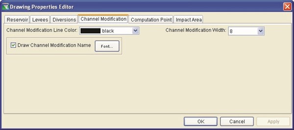
Figure 4.15 Drawing Properties Editor - Channel Modification Tab

The Computation Point tab (Figure 4.16) allows you to select the Fill

Color and Width of the Computation Points. Draw Computation Point Name, when checked, displays the Computation Point names in the display area and does not display when the name is unchecked. The Name Font… button allows you to choose the text font for the names of Computation Points in the watershed display area.

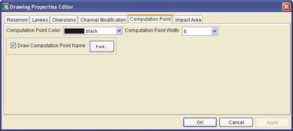
Figure 4.16 Drawing Properties Editor - Computation Point Tab

The Impact Area tab (Figure 4.17) allows you to display or hide the Impact Area name for your watershed. Draw Impact Area Name, when checked, displays Impact Area names on the map and hides the names when unchecked. The Name Font… button allows you to choose the text font for the names of Impact Areas in the watershed display.

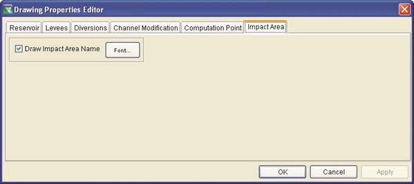
Figure 4.17 Drawing Properties Editor - Impact Area Tab

Impact areas can be included in your ResSim model for consistency with your HEC-FIA model; however, the only computations performed in ResSim are related to the computation points corresponding to the FIA index locations.

For more information about Impact Areas, refer to the HEC-FIA User's Manual (HEC, 2003).

4.4.2 Stream Alignment Layer Properties

When you select Properties for the Stream Alignment layer, the Stream Alignment Properties Editor (Figure 4.18) appears.

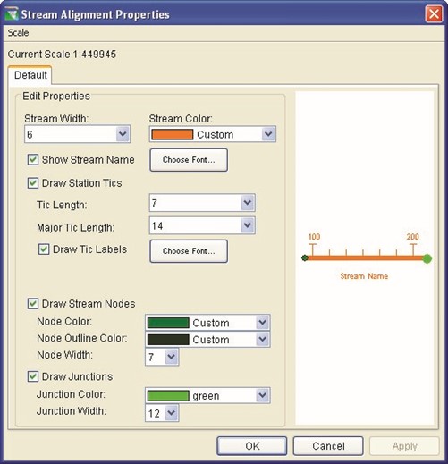
Figure 4.18 Stream Alignment Properties Editor

The Stream Alignment Properties Editor allows you to specify Stream

Width and Stream Color in your watershed display. Show Stream Name, when checked, displays stream names on the map and hides the names when unchecked. The first Choose Font button allows you to choose the text font for the names of streams in the map display. When Draw Station Tics is checked, station tics display on the map, and you are able to specify the Tic Length and Major Tic Length. Draw Tic Labels, when checked, displays Tic labels on the map and hides the labels when unchecked. The second Choose Font button allows you to specify the text font for the Tic Labels. When Draw Station Tics is unchecked, Station Tics do not display on the map and the Tic Length, Major Tic Length, Draw Tic Labels, and Choose Font options are not available.

Similar options are available for Stream Nodes and Stream Junctions (stream junctions occur at the confluence of multiple stream alignments).

The Stream Alignment Properties Editor's preview pane (located on the right side of the editor) allows you to view your changes before applying them.

4.4.3 Map Layers Properties

Map layers can be any of a number of formats supported by ResSim, including ArcView® Shapefiles, AutoCAD® DXF files, raster images,

U.S Geological Survey (USGS) Digital Line Graphs (DLG) files, USGS

Digital Elevation Model (DEM) files, ASCII NET TIN files, and ArcInfo® DEM files. Hence, when you select Properties for a map layer, the editor that opens is specific to the type of map.

For example, if the map layer you wish to configure is a USGS Digital Line Graph map layer, the Properties command opens the USGS Digital Line Graph Editor (Figure 4.19).

Figure 4.19 USGS Digital Line Graph Editor for Digital

Line Graph (DLG) Map Layer, Properties Tab

From the "Properties" tab of this Map Layers Properties Editor, you can specify the default Color of the map and choose whether or not Nodes, Lines, and Areas display in the watershed. You can also set the Saturation and Brightness of the display.

From the "Scale" tab (Figure 4.20) of this Map Layers Properties Editor, you have the choice to Always show the layer, or you can indicate a scale range where the map layer will be visible.

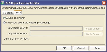
Figure 4.20 USGS Digital Line Graph Editor for Digital Line Graph (DLG) Map Layer, Scale Tab

The directory location of the map file in your ResSim watershed is shown at the top of the dialog box.

Appendix C describes additional map layer editors available in ResSim.

Chapter 5

Working with the Stream Alignment

Table of Contents

Section Page

5 WORKING WITH THE STREAM ALIGNMENT ...................................................... 5-1

5.1 CREATING A NEW STREAM ALIGNMENT .............................................................5 -2 5.2 EDITING AN EXISTING STREAM ALIGNMENT ....................................................... 5-5

5.2.1 MOVING VERTICES OF A STREAM ELEMENT ........................................... 5-5 5.2.2 ADDING VERTICES TO A STREAM ELEMENT ............................................ 5-6 5.2.3 DELETING VERTICES FROM A STREAM ELEMENT .................................... 5-6 5.2.4 EDITING A STREAM ELEMENT ................................................................5 -6 5.2.5 RENAMING A STREAM ELEMENT ............................................................5 -8 5.2.6 DELETING A STREAM ELEMENT .............................................................5 -8 5.2.7 INSERTING A STREAM NODE ................................................................. 5-9 5.2.8 EDITING A STREAM NODE .....................................................................5 -9 5.2.9 DELETING A STREAM NODE ................................................................ 5-10 5.2.10 MOVING A STREAM JUNCTION ............................................................. 5-10 5.2.11 EDITING A STREAM JUNCTION ............................................................. 5-11 5.2.12 REVERSING THE DIRECTION OF A STREAM ........................................... 5-11 5.2.13 DISCONNECTING A STREAM ELEMENT ................................................. 5-12

5.3 IMPORTING A STREAM ALIGNMENT .................................................................. 5-12 5.4 EXPORTING A STREAM ALIGNMENT ................................................................. 5-14 5.5 CONFIGURING STREAM ALIGNMENT DISPLAY PROPERTIES ............................... 5-15 5.6 SAVING THE STREAM ALIGNMENT ................................................................... 5-16 5.7 LISTING OF STREAMS ..................................................................................... 5-16

5-i

List of Figures

Figure Page Number

FIGURE 5.1 STREAM ALIGNMENT ..................................................................................5 -1 FIGURE 5.2 STREAM ELEMENTS ...................................................................................5 -1 FIGURE 5.3 STREAM NODES.........................................................................................5 -1 FIGURE 5.4 STREAM JUNCTIONS ..................................................................................5 -1

FIGURE 5.5 RELATIONSHIP OF LINE SEGMENTS, STREAM ELEMENTS, AND

STREAM ALIGNMENT .............................................................................5 -2 FIGURE 5.6 DRAWING A STREAM ELEMENT ...................................................................5 -3 FIGURE 5.7 CREATE NEW STREAM ...............................................................................5 -4 FIGURE 5.8 CONNECT STREAM REACHES .....................................................................5 -4

FIGURE 5.9 STREAM JUNCTION ....................................................................................5 -4 FIGURE 5.10 MOVING STREAM ELEMENT VERTICES ....................................................... 5-5 FIGURE 5.11 STREAM ALIGNMENT SHORTCUT MENU ..................................................... 5-6

FIGURE 5.12 STREAM EDITOR ......................................................................................5 -7 FIGURE 5.13 ENTER DESCRIPTION - STREAM ELEMENT .................................................. 5-7 FIGURE 5.14 RENAME STREAM .....................................................................................5 -8

FIGURE 5.15 CONFIRMATION MESSAGE WHEN DELETING A STREAM ELEMENT................. 5-8 FIGURE 5.16 STREAM NODE SHORTCUT MENU ..............................................................5 -9 FIGURE 5.17 STREAM NODE EDITOR .............................................................................5 -9 FIGURE 5.18 CONFIRM DELETE OF STREAM NODE ....................................................... 5-10 FIGURE 5.19 MOVING A STREAM JUNCTION ................................................................. 5-10 FIGURE 5.20 STREAM JUNCTION SHORTCUT MENU ...................................................... 5-11 FIGURE 5.21 STREAM JUNCTION EDITOR ..................................................................... 5-11

FIGURE 5.22 CONFIRM REVERSE DIRECTION OF STREAM ELEMENT .............................. 5-12 FIGURE 5.23 IMPORT STREAM ALIGNMENT .................................................................. 5-13

FIGURE 5.24 CHOOSE SHAPEFILE (FOR IMPORTING STREAM ALIGNMENT) ..................... 5-13

5-ii

Chapter 5

Working with the Stream Alignment

The Stream Alignment, illustrated in Figure 5.1, represents the river system in the watershed. It indicates where confluences and bifurcations occur and provides a sense of distance and scale.

Figure 5.1 Stream Alignment

In the Watershed Setup Module, Stream Elements (Figure 5.2), Stream Nodes (Figure 5.3), and Stream Junctions (Figure 5.4) are the components of a Stream Alignment.

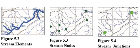
When you create a Stream Alignment, you draw it as a set of connected, multi-segmented lines. The Stream Alignment must have at least two nodes, defining the beginning and end of a stream element. Figure 5.5 illustrates the relationship of line segments, stream elements, and the Stream Alignment.

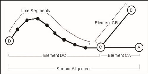
Figure 5.5 Relationship of Line Segments, Stream Elements, and Stream Alignment

ResSim creates and labels stream stations (or river stations) automatically along each stream element. By default, the station at the downstream end of an element is Station 0 (zero), and the stationing increases upstream along the element according to the linear distance between nodes on the stream element in the watershed coordinate system. You can override the default stationing by editing the station values of the stream nodes at the upstream and downstream ends of the stream element, as well as by adding additional nodes along the stream element.

Stream stationing is based on the geographic extents you define when you draw a stream element. If you have set the geographic extents to represent feet, either manually or by importing a layer projected in feet, the station labels will represent feet.

After you have drawn a Stream Alignment in the display area, you can edit, rename, delete, and move its component stream elements, stream nodes, and stream junctions using the Stream Alignment shortcut menus.

5.1 Creating a New Stream Alignment

You must be in the Watershed Setup Module to create a Stream Alignment in ResSim. Although it is not necessary, you will find it useful to display a background map of the river system as a guideline for creating your stream alignment. If your stream alignment is going to be based on a map layer, the map layer should already have been included in the watershed by copying the map files into the "maps" directory. The map layer should contain water features, such as stream channels and reservoirs or lakes. Use this map layer as a guide while creating the stream alignment. By doing this, the units of the labels on the stream alignment will be the same as the units of the water feature layer (i.e., if your water feature layer is projected in state plane coordinates (feet), then the labels on the stream alignment will be in feet). Refer to Chapters 3 and 4 for more information about adding and displaying maps.

You can either digitize a stream alignment by hand or import a stream alignment from an ArcView® shapefile. The following are the steps for digitizing a stream alignment (see Section 5.3 for details on importing a stream alignment).

To create a stream alignment:

You must be in the Watershed Setup Module. On the Module list, select Watershed Setup.
On the map toolbar, press the Stream Alignment Tool .
Determine an upstream location where you want to start a stream element (typically, you will begin at the upstream end of the mainstem and end at the most downstream location of the primary river in your watershed).
Hold down the CTRL key. Starting at the upstream end, draw the stream element by clicking the left mouse button at each vertex point as illustrated in Figure 5.6.

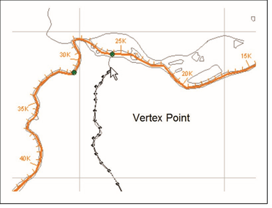
Figure 5.6 Drawing a Stream Element
Continue downstream (while continuing to hold down the CTRL key) and before placing the last point of the stream element, release the CTRL key, and then click the left mouse button at the last downstream location. This creates the ending stream node of the stream element.
The Create New Stream dialog box (Figure 5.7) opens. You can either accept the default name or enter a new name. Also, you can enter a description for the stream element. Click OK to close the Create New Stream dialog box.

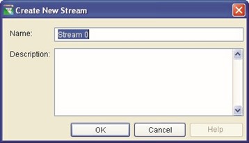
Figure 5.7 Create New Stream

Repeat steps 4 through 6 to add more stream elements to your stream alignment.
To create a confluence or bifurcation, end the stream element by clicking directly on an existing stream element. After naming the new stream element, the Connect Stream Reaches dialog box (Figure 5.8) will appear. You need to determine whether you want to connect the new stream element to the existing stream element. Click Yes if you want the two stream elements connected; otherwise click No. If you selected No, and if there are additional existing streams that are possible candidates for connecting your new stream element to, then a subsequent Connect Stream Reaches dialog will appear to give you the opportunity to connect to the existing stream.

Figure 5.8 Connect Stream Reaches

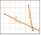
When multiple stream elements are connected (e.g., at a confluence), a stream junction is automatically created and appears as a highlighted green circle (a "light green halo") as shown

^{in Figure 5.9.}Figure 5.9 Stream Junction

Once you have completed the creation of your stream alignment, save your work. From the File menu, select Save Watershed and the stream alignment for your watershed will be saved.

5.2 Editing an Existing Stream Alignment

After drawing a stream alignment in the display area, there are many options available for revising your stream alignment. To edit your stream alignment, you must be in the Watershed Setup Module. The Zoom Tool can be used to help magnify the stream network, thus providing more detail to make editing the stream alignment easier.

This section describes the following capabilities for editing your Stream Alignment:

how to refine and re-shape your stream alignment (by moving/adding/deleting vertex points of the stream elements)
how to review stream stationing and provide a stream element description (by using the stream element editor)
how to rename and delete stream elements
how to add and edit stream nodes (for defining stream stationing)
how to move and edit stream junctions
how to reverse the flow direction of a stream element
how to disconnect a stream element

Since the Stream Alignment may be referenced by other models, care should be used when making any changes to it.

5.2.1 Moving Vertices of a Stream Element

To move a vertex of an existing Stream Element:

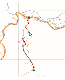Lockthe
configuration.
With the Stream
Alignment Tool selected, double-click anywhere on the stream element. The stream element you select will turn red and all the vertices of that stream element will turn blue.
Click on the vertex you want to move, and drag
it to a new location, as
illustrated in Figure
Figure 5.10 Moving Stream 5.10.

Element Vertices

5.2.2 Adding Vertices to a Stream Element

To add vertex points to an existing stream element:

Lockthe configuration.
With the Stream Alignment Tool selected, double-click anywhere on the stream element. The stream element you select will turn red and all the vertices of that stream element will turn blue.
Place the pointer on the selected stream element where you want to add a vertex point. Hold down the CTRL key and click. A blue point will appear on the selected stream where you have added a vertex point.

5.2.3 Deleting Vertices from a Stream Element

To delete vertex points from an existing stream element:

Lockthe configuration.
With the Stream Alignment Tool selected, double-click anywhere on the stream element. The stream element you select will turn red and all the vertices of that stream element will turn blue.
Hold down the SHIFT+CTRL keys and click on the vertex point to be deleted. The blue vertex point will disappear from the stream element, and the stream will straighten between the two adjacent vertices.

5.2.4 Editing a Stream Element

To edit a Stream Element:

Lockthe configuration.
With the Stream Alignment Tool selected, right-click on the stream you want to edit.
From the shortcut menu
(Figure 5.11), select Edit Stream Element to open the Stream Editor (Figure 5.12).

Figure 5.11 Stream Alignment

Shortcut Menu

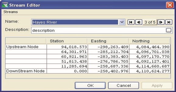
Figure 5.12 Stream Editor

The Stream Editor displays a summary of the stream name, description, stationing, and coordinates for a stream element. You can edit only the description.

Stream name:

The Stream Editor displays the name of the Stream Element you have selected in the list along with all available Stream Elements in the watershed. Also, left and right arrows (navigator buttons) allow you to click through the Stream Elements in the watershed.

Description:

To edit the Description of the Stream Element, you can type into the text area or click the button to access the Enter Description dialog box (Figure 5.13)

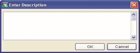
Figure 5.13 Enter Description - Stream Element

Stationing:

The Stream Editor provides you with a report of the stream stationing and coordinates of the Upstream and Downstream nodes, plus any stream nodes in between them. Use the Stream Node Editor

(described in Section 5.2.8) to edit the stream stationing of the nodes.

5.2.5 Renaming a Stream Element

To rename a stream element:

Lock the configuration.
With the Stream Alignment Tool selected, right-click on the stream element and select Rename Stream Element.
Enter a new Name and Description for the stream element in the Rename Stream dialog box illustrated in Figure 5.14.

Figure 5.14 Rename Stream

5.2.6 Deleting a Stream Element

To delete a stream element:

Lock the configuration.
With the Stream Alignment Tool selected, right-click on the stream element and select Delete Stream Element.
When the confirmation message (shown below in Figure 5.15) appears, select either Yes or No.

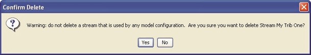
Figure 5.15 Confirmation Message when Deleting a Stream Element

It is important to remember that other models (e.g., HEC-FIA) may use the same stream alignment, so be sure to confirm with other modelers before deleting any stream elements.

5.2.7 Inserting a Stream Node

By default, ResSim generates beginning and ending stream nodes for each stream element. Also, stream nodes are automatically created where stream elements connect (stream junctions). Since stream nodes are used for establishing the stream stationing, you may want to include additional stream nodes along your stream element for locations where you want to define specific stream stationing.

It is important to keep in mind when defining the stream

stations that the locations you specify for stationing are common to all models that use stationing in their computations.

To insert a stream node on an existing Stream Alignment:

Lock the configuration.
Using the Stream Node Tool , hold down the CTRL key and right-click on the Stream Alignment in the place where the stream node is to be inserted.
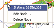When you right-click on the stream station node, a shortcut menu appears (Figure 5.16).
From the shortcut menu on the stream node, you can Figure 5.16 Stream Node choose Edit Node, which Shortcut Menu will bring up the Stream

Node Editor illustrated in Figure 5.17.

5.2.8 Editing a Stream Node

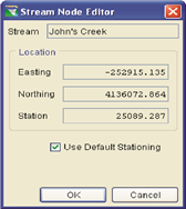The Stream Node Editor (Figure 5.17) displays the location information for the node.

The Use Default Stationing check box is selected by default. When you select this option, the current location of the selected node displays in the Stream Node Editor.
If you want to specify the exact location for the node on the stream

element, then "deselect" the

Use Default Stationing to make Figure 5.17 Stream the Station box editable. Node Editor

Enter the location for the station directly into the Station box, and then click OK.

5.2.9 Deleting a Stream Node

Since stream nodes define the stream stationing that may be referenced by other models, care should be used when deleting stream nodes.

To delete a stream node from an existing Stream Alignment:

Lock the configuration.
Find the stream node you wish to delete.
Using the Stream Node Tool , right-click on the stream node.
Select Delete Node from the shortcut menu.
A Confirm Delete message will display (Figure 5.18) asking you whether you really
want to delete the selected stream node.
Click Yes and the Figure 5.18 Confirm Delete of message will close and Stream Node the stream node will be deleted from the stream element.

5.2.10 Moving a Stream Junction

When two stream elements intersect (e.g., at a confluence), a Stream Junction is automatically created. A stream junction is multiple stream nodes at one location and is represented by a dark green circle with a light green halo around the circle. Although ResSim generates default stream junctions when you create the Stream Alignment, you can move them as needed.

To move a Stream Junction along an existing Stream Alignment:

Lock the configuration.
With the Stream Node Tool

selected, double-click on

the stream junction. The stream junction you select will turn dark green and will have small squares (handles) at each corner (Figure 5.19).

To move the stream junction, click and drag it along the stream element to its new position.

Figure 5.19 Moving a

Stream Junction

5.2.11 Editing a Stream Junction

To edit a Stream Junction:

Lock the configuration.
Using the Stream Node

Tool , right-click on

the Stream Junction to Figure 5.20 Stream Junction access the shortcut menu Shortcut Menu

(Figure 5.20).

Select Edit Junction to open the Stream Junction Editor (Figure 5.21).

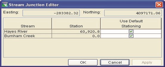
Figure 5.21 Stream Junction Editor

The Stream Junction Editor displays the list of stream nodes associated with a junction and allows you to edit the stationing of each of the nodes by deselecting the "Use Default Stationing" box and entering the desired station.

5.2.12 Reversing the Direction of a Stream

If you find that you have inadvertently drawn your stream element in the wrong direction (e.g., downstream to upstream when it should be upstream to downstream), then instead of having to delete the stream element and redraw it, you can choose to reverse the direction of the stream element.

To reverse the direction of a stream element:

Lock the configuration.
With the Stream Alignment Tool selected, right-click on the stream element and select Reverse Direction from the shortcut menu.
A warning message (Figure 5.22) will open asking you whether you really want to reverse the direction of the stream element.

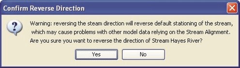
Figure 5.22 Confirm Reverse Direction of Stream Element

Click Yes and the warning message will close and the stream element's direction will be reversed.

5.2.13 Disconnecting a Stream Element

A stream element can be connected to another stream element (e.g., at the confluence of two streams). If, for some reason, you need to disconnect the stream element from another stream element, you can do so.

To disconnect a stream element from another stream element:

Lock the configuration.
With the Stream Alignment Tool selected, right-click on the stream element you want to disconnect and select either Disconnect Upstream or Disconnect Downstream, as appropriate, from the shortcut menu.
The stream element will now be disconnected from the other stream element. On the display area, the upstream (or downstream) point will physically move away from the connecting stream element and a stream node will remain where the stream element was originally connected.

5.3 Importing a Stream Alignment

To import a stream alignment you must first have as an active map layer

(see "Adding a New Map Layer" in Chapter 3, Section 3.4.2) an ArcView® shapefile which represents the stream system of your watershed. This shapefile must have an attribute that is the name of each stream, and each stream must form a contiguous line with one upstream point and one downstream point.

To import a stream alignment:

You must be in the Watershed Setup Module. From the Module list, select Watershed Setup.
Add the map layer that will be imported to the display area (see "Adding a New Map Layer" in Chapter 3, Section 3.4.2 to add a map layer).
From the Watershed menu, point to Import, and then select Stream Alignment.
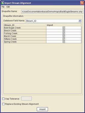The Import Stream
Alignment dialog box
(Figure 5.23) will open.

In the Shapefile Name box is displayed one of the ArcView® shapefiles defined as active map layers in your watershed. ResSim automatically selects the first shapefile that contains polylines. Therefore, if this is not the desired shapefile,
then from the File menu, select Choose Shapefile.

Figure 5.23 Import Stream

Alignment

The Choose Shapefile dialog box (Figure 5.24) will open. In the Available box is a list of the available polyline shapefiles that you have added as map layers. In the Selected box is the polyline shapefile that has been chosen. To choose a different polyline shapefile, use the Add and Remove buttons to get the correct shapefile. In Figure 5.24, the polyline shapefile to be used for importing the stream alignment is BaldEagleRivers.shp.

Figure 5.24 Choose Shapefile

(for Importing Stream Alignment)

Once the correct shapefile has been chosen, the required attribute is the name of each stream. The program automatically searches for a database field name of
Stream_ID. If there is not a database field name of Stream_ID, then in the Database Field Name list, you must select the database field name that contains the names of each stream. In the example shown in Figure 5.23, for the shapefile BaldEagleStreams.shp, the database field name is Stream_ID.
When you have selected the correct database field name, the table will list the stream names. If each stream is a contiguous line with one upstream point and one downstream point, then the checkbox in the Import column of the table will be set. If there is something wrong with the line that represents a stream, the checkbox will not be set, and ResSim will not import that stream element.
Gap Tolerance (Figure 5.23) is used to connect stream elements that have a gap between the end point and the junction with another stream. By default, the Gap Tolerance is set to zero (0.0), so ResSim can connect streams to other streams. If you click Gap Tolerance, then you need to enter a value larger than zero in the Gap Tolerance box, which will allow ResSim to connect streams that might have a larger gap between them.
The Replace Existing Stream Alignment box, allows you to replace the existing stream alignment with the one being imported from the selected ArcView® shapefile.
Once everything is set, click Import. The stream alignment will be automatically drawn in the display area. From the File menu, choose Close and the Import Stream Alignment dialog box (Figure 5.23) will close.

5.4 Exporting a Stream Alignment

If you have digitized a stream alignment by hand, you might want to save that stream alignment as an ArcView® shapefile. To export a stream alignment you must have a stream alignment in the display area.

To export a stream alignment:

You must be in the Watershed Setup Module. On the Module list, click Watershed Setup.
From the Watershed menu, point to Export, and then select Stream Alignment.
A Save File browser (Figure 5.25) will open. Enter a name in the File Name box. Click OK, the Save File browser will close, and you will have an ArcView® shapefile of the displayed stream alignment.

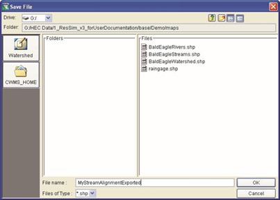
Figure 5.25 Save File Browser

5.5 Configuring Stream Alignment Display Properties

You can change the color, line width, font, and tic mark properties of a Stream Alignment using the Stream Alignment Properties Editor. The section on "Viewing and Configuring Layer Properties" in Chapter 4, Section 4.4 describes in detail how to change Stream Alignment display properties.

To change stream alignment properties:

From the View menu, select Layers.
The Layer Selector dialog box will open.
Right-click on the StreamAlignment layer in the tree. From the shortcut menu, click Properties.
The Stream Alignment
Properties dialog box (Figure 5.26) will open.
To change the color of the stream alignment layer, select a color from the Stream Color list. The preview pane to the right of the Edit Properties box will display the selected color.

Figure 5.26 Stream Alignment

Properties

Click OK and the Stream Alignment Properties dialog box will close and the color change will appear in the display area.
Repeat steps 5 and 6 for any other changes you wish to make to the stream alignment properties.
Once you have finished, from the Layer Selector dialog box, click OK to close.

Saving the Stream Alignment

Since creating a stream alignment can be a very detailed activity, you should save it frequently during its creation. From the File menu, click Save Watershed. This command will save all of the stream alignment properties and the appropriate files created and used by ResSim for the stream alignment.

Listing of Streams

Once you have your stream alignment completed, it's a good idea to review the streams in your stream alignment. From the Watershed Setup Module, there is a report that contains this information.

From the Reports menu, select List of Streams and a report similar to Figure 5.27 will appear.

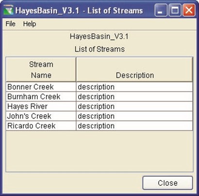
Figure 5.27 List of Streams in Stream Alignment

This report provides a list of streams and their descriptions that have been input for the stream alignment.
From the File menu of the report, you can print the report, or you can export the report as an ASCII tab-delimited file.
Click Close and the List of Streams report will close.

Chapter 6

Creating Watershed Elements

Table of Contents

Section Page

6 CREATING WATERSHED ELEMENTS ................................................................. 6 1

6.1 CREATING A RESERVOIR ..................................................................................6 1

6.1.1 EDITING RESERVOIR DATA (WATERSHED SETUP) .................................. 6 2

6.1.2 RENAMING A RESERVOIR ......................................................................6 3

6.1.3 REMOVING A RESERVOIR FROM A CONFIGURATION ................................ 6 4

6.1.4 DELETING A RESERVOIR .......................................................................6 4

6.1.5 ADDING CONFIGURATION NOTES FOR A RESERVOIR............................... 6 4

6.2 CREATING A LEVEE ..........................................................................................6 5

6.2.1 EDITING LEVEE DATA ...........................................................................6 5

6.2.2 RENAMING A LEVEE..............................................................................6 7

6.2.3 REMOVING A LEVEE FROM A CONFIGURATION ........................................ 6 7

6.2.4 DELETING A LEVEE ...............................................................................6 8

6.2.5 ADDING CONFIGURATION NOTES FOR A LEVEE ...................................... 6 8

6.3 CREATING A DIVERSION ...................................................................................6 9

6.3.1 EDITING DIVERSION DATA .................................................................. 6 10

6.3.2 RENAMING A DIVERSION ..................................................................... 6 10

6.3.3 DISCONNECTING A DIVERSION ............................................................ 6 11

6.3.4 REMOVING A DIVERSION FROM A CONFIGURATION ............................... 6 11

6.3.5 DELETING A DIVERSION ...................................................................... 6 11

6.3.6 ADDING CONFIGURATION NOTES FOR A DIVERSION .............................. 6 12

6.4 CREATING CHANNEL MODIFICATIONS .............................................................. 6 12

6.4.1 EDITING CHANNEL MODIFICATION DATA .............................................. 6 13

6.4.2 RENAMING A CHANNEL MODIFICATION ................................................. 6 13

6.4.3 REMOVING A CHANNEL MODIFICATION FROM A CONFIGURATION ........... 6 14

6.4.4 DELETING A CHANNEL MODIFICATION .................................................. 6 14

6.4.5 ADDING CONFIGURATION NOTES FOR CHANNEL MODIFICATIONS .......... 6 14

6.5 CREATING OFF-CHANNEL STORAGE AREAS .................................................... 6 15

6.5.1 EDITING OFF-CHANNEL STORAGE DATA .............................................. 6 15

6.5.2 RENAMING AN OFF-CHANNEL STORAGE AREA ..................................... 6 16

6.5.3 REMOVING AN OFF-CHANNEL STORAGE AREA FROM A CONFIGURATION ........................................................................ 6 16

6.5.4 DELETING AN OFF-CHANNEL STORAGE AREA ...................................... 6 17

6.5.5 ADDING CONFIGURATION NOTES FOR AN OFF-CHANNEL STORAGE AREA ..................................................... 6 17

6 i

6.6 CREATING "OTHER" PROJECTS....................................................................... 6-18

6.6.1 EDITING "OTHER" PROJECT DATA ....................................................... 6-18 6.6.2 RENAMING "OTHER" PROJECTS .......................................................... 6-19

6.6.3 REMOVING "OTHER" PROJECTS FROM A CONFIGURATION ..................... 6-19

6.6.4 DELETING "OTHER" PROJECTS ........................................................... 6-20

6.6.5 ADDING CONFIGURATION NOTES FOR "OTHER" PROJECTS ................... 6-20

6.8.1 EDITING COMPUTATION POINT DATA ................................................... 6-21

6.8.2 RENAMING A COMPUTATION POINT AND EDITING THE DESCRIPTION ...... 6-23

6.8.3 DELETING A COMPUTATION POINT ...................................................... 6-23 6.9 WORKING WITH TIME-SERIES ICONS ............................................................... 6-24

List of Figures

Figure Page Number

FIGURE 6.1 RESERVOIR ELEMENTS IN WATERSHED SETUP MODULE .............................. 6-1 FIGURE 6.2 NAME NEW RESERVOIR .............................................................................6 -2 FIGURE 6.3 RESERVOIR PROPERTIES EDITOR ...............................................................6 -3 FIGURE 6.4 WARNING MESSAGE WHEN RENAMING RESERVOIR ...................................... 6-3 FIGURE 6.5 CONFIRM REMOVAL OF RESERVOIR ............................................................6 -4 FIGURE 6.6 CONFIGURATION NOTES FOR RESERVOIR ................................................... 6-4 FIGURE 6.7 LEVEE DRAWING ........................................................................................6 -5 FIGURE 6.8 LEVEE PROPERTIES EDITOR .......................................................................6 -6 FIGURE 6.9 WARNING MESSAGE WHEN RENAMING LEVEE ............................................. 6-7 FIGURE 6.10 CONFIRM REMOVAL OF LEVEE ..................................................................6 -7 FIGURE 6.11 CONFIGURATION NOTES FOR LEVEE ..........................................................6 -8 FIGURE 6.12 EXAMPLE DIVERSIONS ..............................................................................6 -9 FIGURE 6.13 DIVERSION EDITOR ................................................................................. 6-10

FIGURE 6.14 WARNING MESSAGE WHEN RENAMING DIVERSIONS ................................. 6-10

FIGURE 6.15 DIVERSION SHORTCUT MENU DISCONNECT OUTFLOW.............................. 6-11 FIGURE 6.16 CONFIGURATION NOTES FOR DIVERSION ................................................. 6-12 FIGURE 6.17 CHANNEL MODIFICATION EDITOR ............................................................ 6-13 FIGURE 6.18 WARNING MESSAGE WHEN RENAMING CHANNEL MODIFICATION ............... 6-13 FIGURE 6.19 CONFIGURATION NOTES FOR CHANNEL MODIFICATION ............................. 6-14 FIGURE 6.20 OFF-CHANNEL STORAGE EDITOR ............................................................ 6-15

Chapter 6

Creating Watershed Elements

In the Watershed Setup Module you can define the Projects and Computation Points used in ResSim.

ResSim provides the tools for drawing geographically referenced Projects including Reservoirs, Levees, Diversions, Channel Modifications, OffChannel Storage Areas, and "Other" Projects. The tools provide the ability to edit the graphical representation of the Project within the map display panel, and they also provide access to menu items for editing the Project data directly from the map display. ResSim computations include only reservoir and diversion projects.

When you add a Project to the map display panel, it becomes part of the Configuration you currently have selected. A "superset" of all configurations is named "Study" and includes all of the Projects for the watershed. For more information on associating projects with Configurations, refer to Chapter 7.

The Computation Point set contains all locations where time-series information is to be computed for possible exchange between application models (e.g., ResSim and FIA). ResSim automatically generates

Computation Points when Projects are placed on the Stream Alignment.

6.1 Creating a Reservoir

You will create a reservoir by starting at the upstream end of the reservoir.

After the reservoir has been created, several visual elements will appear (as shown in Figure 6.1) that represent a reservoir: a storage reach (cyan), a "pool" (cyan triangle), a "dam" (small gray rectangle), and computation points (black dots) at the upstream and downstream locations of the reservoir on the stream alignment.

Setup Module

To add a reservoir to the watershed:

Select the Reservoir Tool .
While holding down the CTRL key, click on the stream alignment at the upstream location of the reservoir. If more than one stream flows into the reservoir pool, continue holding down the CTRL key and click at each location of inflow into the reservoir on these streams.
Release the CTRL key and click on the stream alignment at the downstream location of the reservoir (where the dam is located). Reservoirs should not overlap previously placed computation points.
When you release the mouse button after creating the downstream end of the reservoir, the Name New Reservoir dialog box appears (Figure 6.2).

Figure 6.2 Name New Reservoir

You name the Reservoir by typing a name in the Name field.

Optionally, you can enter a Description for the Reservoir.

Click OK when you are done.

The new Reservoir will now appear in your map display.

6.1.1 Editing Reservoir Data (Watershed Setup)

To edit data for the Reservoir in the Watershed Setup Module, select

the Reservoir Tool and right-click on the Reservoir. From the shortcut menu, select Edit Reservoir to access the Reservoir Editor (Figure 6.3).

Figure 6.3 Reservoir Properties Editor

In the Watershed Setup Module, the only data that you need to specify for the Reservoir is its Name and Label Position (additional data is entered in the Reservoir Network Module). The Label Position selects where to place the reservoir name in the display area, relative to the reservoir.

Check Existing Project if the reservoir currently exists so that the reservoir will be added automatically to any new configurations. You can remove it at any time by selecting Remove from Configuration in the shortcut menu or by using the Configuration Editor. This is a useful option if you are creating multiple configurations that use the same set of reservoirs.

Certain models compute project benefits (e.g., HEC-FIA); therefore, use the Corps Projects checkbox to indicate if the reservoir is a Corps Project.

The Year in Service field is optional and is used in planning studies. You do not need to specify a year in service when defining projects for real-time studies.

6.1.2 Renaming a Reservoir

To rename a Reservoir, select the Reservoir Tool and right-click on the Reservoir. From the shortcut menu, select Rename Reservoir. This command opens a dialog box that allows you to rename the reservoir. A warning message (Figure 6.4) appears when you save the new name, asking you to confirm that you want to rename the reservoir. If you choose to rename the reservoir,

remember that changing a

reservoir name may affect one or more of the configurations

Figure 6.4 Warning Message

that recognize the reservoir.

when Renaming Reservoir

6.1.3 Removing a Reservoir from a Configuration

To remove a Reservoir from the current Configuration, select the

Reservoir Tool and right-click on the Reservoir. From the shortcut menu, select Remove from Configuration. This command removes the reservoir from the Configuration that is currently displayed in the Configuration box on the toolbar. The Confirm Removal dialog box appears (Figure 6.5).

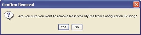
Figure 6.5 Confirm Removal of Reservoir

You can also remove a Reservoir from a Configuration by accessing the Configuration Editor and manually removing the reservoir from the Projects tab using the Project Selector.

6.1.4 Deleting a Reservoir

To delete a Reservoir from the watershed, select the Reservoir Tool and right-click on the Reservoir. From the shortcut menu, select Delete Reservoir. This command removes the reservoir and all data associated with the reservoir from the watershed. You are asked to confirm a deletion before the reservoir is removed, and asked if you would like to delete the reservoir's computation points. If you choose to delete the reservoir, remember that deleting the reservoir may affect one or more of the configurations that recognize the reservoir.

6.1.5 Adding Configuration Notes for a Reservoir

To add Configuration Notes for a Reservoir, select the

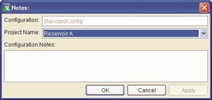Reservoir Tool and right-click on the Reservoir. From the shortcut menu, select Configuration Notes. This

command opens a dialog

box (Figure 6.6) for

Figure 6.6 Configuration Notes

entering text information

for Reservoir

about a project specific to the configuration.

6.2 Creating a Levee

A levee is an earthen barrier built along a stream to provide protection from flooding. A levee can reduce flood damage by preventing flood stages from reaching a potential damage area.

To add a levee to the watershed:

Select the Levee Tool .
While holding down the CTRL key, click on the stream alignment to select the upstream end of the levee, then release the CTRL key and click to select the downstream end.

When you release the mouse button after clicking at the downstream end of the levee, a dialog box appears for you to provide a name and description. After entering a Levee name, the levee will be drawn as a black line following the stream alignment. However, using the Levee Editor (see Follows Stream option in Section 6.2.1), you can allow for positioning the levee along the side of the stream alignment in the display area (Figure 6.7).

6.2.1 Editing Levee Data

To edit Levee data, right-click on the levee and select Edit Levee. The Levee Properties Editor opens, as shown in Figure 6.8.

In addition to the Levee Name and Description, the Levee Editor displays the Stream Name and the Start and End Stations for the levee. You can edit the stationing manually by directly entering values in the Start Station and End Station fields.

The Follows Stream checkbox is selected by default. With this option selected, the levee is drawn in parallel to the stream alignment. By deselecting the Follows Stream checkbox, you can allow for moving the levee and editing its shape using the Levee Tool in the map display. To do this, first double-click the levee to select it. The levee will turn yellow and the beginning and end points will appear as black dots. To add additional vertex points, CTRL-click along the levee. You can then drag any of the vertex points to the desired location. This process is very similar to editing the stream alignment, with the exception of the mouse tool used.

Certain models compute project benefits (e.g., HEC-FIA); therefore, use the Corps Projects checkbox to indicate if the levee is a Corps Project.

ResSim does not actually use levees in its computations. However, those models that do use levee data in their computations contain the tools for configuring the levee data. Therefore, refer to the appropriate model's User's Manual (e.g., HEC-FIA) for further information.

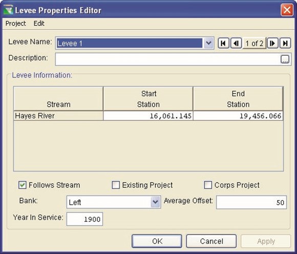
Figure 6.8 Levee Properties Editor

6.2.2 Renaming a Levee

To rename a Levee:

Select the Levee Tool and right-click on the Levee.
From the shortcut menu, select Rename Levee. This command opens a dialog box that allows you to rename the levee.
If you choose to rename the levee, remember that changing the levee name may affect one or more of the configurations that recognize the levee.
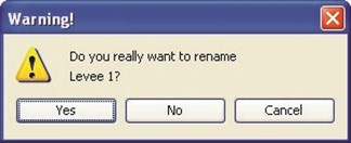A warning message appears (Figure 6.9) when you save the new
name, asking you
to confirm that you want to rename the Figure 6.9 Warning Message levee. when Renaming Levee

6.2.3 Removing a Levee from a Configuration

To remove a Levee from the current Configuration:

1. Select the Levee Tool 2. Right-click on the Levee.

3. From the shortcut menu, select Remove from Configuration. This command removes the levee from the Configuration that is currently displayed in the Configuration box on the toolbar. The Confirm Removal dialog box appears (Figure 6.10).

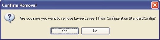
Figure 6.10 Confirm Removal of Levee

You can also remove a Levee from a Configuration by accessing the

Configuration Editor and manually removing the levee from the Projects tab using the Project Selector.

6.2.4 Deleting a Levee

To delete a Levee from the watershed:

Select the Levee Tool .
Right-click on the Levee.
From the shortcut menu, select Delete Levee. This command removes the levee and all data associated with the levee from the watershed. You are asked to confirm a deletion before the levee is removed. Again, if you choose to delete the levee, remember that deleting the levee may affect one or more of the configurations that recognize the levee.

6.2.5 Adding Configuration Notes for a Levee

To add Configuration Notes for a Levee:

Select the Levee Tool and right-click on the Levee.
From the shortcut menu, select Configuration Notes. This command opens a dialog box (Figure 6.11) for entering text information about a project that is specific to the configuration.

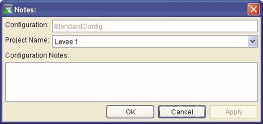
Figure 6.11 Configuration Notes for Levee

6.3 Creating a Diversion

To add a Diversion to the watershed:

Select the Diversion Tool .
While holding down the CTRL key, click to select the location on the stream alignment where the diversion will occur (the "from" location). Then, release the CTRL key and click to select the location where the diverted water will go (the "to" location). The "to" location (location that will receive the diverted water) can be on the stream alignment (which indicates that the diverted water will remain within the channel system) or it can be a point in the display area that is not connected to the stream alignment (which will indicate a loss of the diverted water to the channel system).
When you release the mouse button after creating the diversion, a dialog box appears for you to provide a name and description.
After entering a name, the Diversion is drawn in the display area. If both ends of the diversion are connected to the stream alignment, then Computation Points are automatically generated at each end of the diversion (the color of the arrow head will be blue). If the diversion is only connected to the stream alignment at the location where the water is diverted from, then a
Computation Point will be generated at that location only (and the color of the arrow head will be black).
It's a good idea to rename the Computation Points that are automatically generated for a diversion. To do this, select the
Computation Point Tool and right-click on the computation points at the ends of the diversion. Then, from the shortcut menu, select Rename Computation Point. Figure 6.12 shows example diversions where the Computation Points for the diversions were renamed ("PutDiv", "GetDiv", and "DivOut").

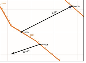After the diversion is defined, it will show up as a black line with an arrow head at the divert-to end. If the diversion leaves one location and returns to another location (see "MyDiv" diversion in Figure 6.12), the arrow head is blue. If the diversion leaves the system (see "YourDiv" diversion in

Figure 6.12), then the arrow

Figure 6.12 Example Diversions

head is displayed in black instead of blue.

6.3.1 Editing Diversion Data

To edit Diversion Data:

Select the Diversion Tool .
Right-click on the Diversion and select Edit Diversion. The Diversion Editor opens, as shown in Figure 6.13.

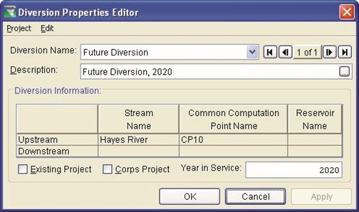
Figure 6.13 Diversion Editor

The Diversion Editor is similar to the Reservoir Editor described in

Section 6.1.1. You can specify whether the diversion is an Existing Project, a Corps Project, and the Year in Service (as previously described in Section 6.1.1). The Stream and the Computation Point names that the diversion connects to are also shown.

6.3.2 Renaming a Diversion

To rename a Diversion

Select the Diversion Tool .
Right-click on the Diversion and from the shortcut menu select Rename Diversion. This command opens a dialog box that allows you to rename the diversion. If you choose to rename the diversion, remember that changing the diversion name may affect one or more of the configurations that recognize the diversion.
A warning message (Figure 6.14) appears when you save the new name,
asking you to

confirm that you

want to rename the Figure 6.14 Warning Message when diversion. Renaming Diversions

6.3.3 Disconnecting a Diversion

If you decide to disconnect the outflow of a diversion:

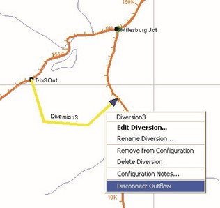Select the Diversion Tool
.
Right-click on a Diversion that is connected to another location and select Disconnect Outflow from the shortcut menu (Figure 6.15).

Figure 6.15 Diversion Shortcut Menu Disconnect Outflow

6.3.4 Removing a Diversion from a Configuration

To remove a Diversion from the current Configuration:

Select the Diversion Tool .
Right-click on the Diversion and from the shortcut menu select Remove from Configuration. This command removes the diversion from the Configuration that is currently displayed in the Configuration box on the toolbar. The Confirm Removal dialog box will appear.

You can also remove a Diversion from a Configuration by accessing the Configuration Editor and manually removing the diversion from the Projects tab using the Project Selector.

6.3.5 Deleting a Diversion

To delete a Diversion from the watershed:

Select the Diversion Tool and right-click on a Diversion.
From the shortcut menu, select Delete Diversion. This command removes the diversion and all data associated with the diversion from the watershed. You are asked to confirm a deletion before the diversion is removed. Again, if you choose to delete the diversion, remember that deleting the diversion may affect one or more of the configurations that recognize the diversion.

6.3.6 Adding Configuration Notes for a Diversion

To add Configuration Notes for a Diversion:

Select the Diversion Tool and right-click on the Diversion.
From the shortcut menu, select Configuration Notes. This command opens a dialog box (Figure 6.16) for entering text information about a diversion that is specific to the configuration.

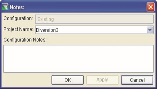
Figure 6.16 Configuration Notes for Diversion

6.4 Creating Channel Modifications

To add a Channel Modification to the watershed:

Select the Channel Modification Tool .
Hold down the CTRL key and click at the upstream end of the channel modification along the stream alignment.
Release the CTRL key and click on the downstream end of the channel modification.

When you release the mouse button after creating the downstream end, the channel modification is drawn along the stream alignment and a dialog box appears for you to provide a name and description. After entering a name, the channel modification is drawn along the stream alignment in the display area. Note that Channel Modifications are not yet implemented in ResSim's computations.

6.4.1 Editing Channel Modification Data

To edit Channel Modification Data:

Select the Channel Modification Tool .
Right-click on the Channel Modification and select Edit Channel Modification. The Channel Modification Editor opens, as shown in Figure 6.17.

Figure 6.17 Channel Modification Editor

The Channel Modification Editor contains the basic configuration data for the Channel Modification Project, such as whether it is an Existing Project, a Corps Project, the Label Position, the Stream Name, and the Year in Service (as previously described in Section 6.1.1).

6.4.2 Renaming a Channel Modification

To rename a Channel Modification:

Select the Channel Modification Tool and right-click on the Channel Modification.
From the shortcut menu, select Rename Channel
Modification. This command opens a dialog box that allows you to rename the channel modification. If you choose to rename the channel modification, remember that changing the name may affect one or more of the configurations that recognize the channel modification.
A warning message (Figure 6.18) appears when you save the new name, asking
you to confirm that
you want to rename

the channel Figure 6.18 Warning Message when modification. Renaming Channel

Modification

6.4.3 Removing a Channel Modification from a Configuration

To remove a Channel Modification from the current Configuration:

Select the Channel Modification Tool and right-click on the Channel Modification.
From the shortcut menu, select Remove from Configuration. This command removes the Channel Modification from the Configuration that is currently displayed in the Configuration box on the toolbar. The Confirm Removal dialog box appears.

You can also remove a Channel Modification from a Configuration by accessing the Configuration Editor and manually removing the Channel Modification from the Projects tab using the Project Selector.

6.4.4 Deleting a Channel Modification

To delete a Channel Modification from the watershed:

Select the Channel Modification Tool and right-click on the Channel Modification.
From the shortcut menu, select Delete Channel Modification. This command removes the Channel Modification and all data associated with it from the watershed. You will be asked to confirm a deletion before the Channel Modification is removed. Again, if you choose to delete the Channel
Modification, remember that deleting it may affect one or more of the configurations that recognize the project.

6.4.5 Adding Configuration Notes for Channel Modifications

To add Configuration Notes for a Channel Modification:

Select the Channel Modification
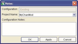Tool and right-click on the Channel Modification.
From the shortcut menu, select Configuration Notes. This
command opens a dialog box

(Figure 6.19) for entering text

information about a project that is specific to the configuration.

Figure 6.19 Configuration

Notes for Channel Modification

6.5 Creating Off-Channel Storage Areas

To add an Off-Channel Storage Area to the watershed:

Select the Off-Channel Storage Tool .
Hold down the CTRL key and click the location in the map where you want to add the Storage Area. Continue to hold the CTRL key while you click to add additional vertex points for the bounding polygon that represents the Off-Channel Storage Area.
When you reach the end point, release the CTRL key and click to place the last point.
When you release the mouse button, a dialog box appears for you to provide a name and description. After entering a name, the polygon appears in the map display area. Note that Off-Channel Storage Areas are not yet implemented in ResSim's computations.

6.5.1 Editing Off-Channel Storage Data

To edit Off-Channel Storage data:

Select the Off-Channel Storage Tool and right-click on the Off-Channel Storage Area.
Select Edit Off-Channel Storage. The Off-Channel Storage Editor opens, as shown in Figure 6.20.

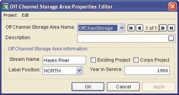
Figure 6.20 Off-Channel Storage Editor

The Off-Channel Storage Editor contains the basic configuration data for the Off-Channel Storage project, such as whether the project is an

Existing Project, a Corps Project, the Label Position, the Stream Name, and the Year in Service (as previously described in Section 6.1.1).

6.5.2 Renaming an Off-Channel Storage Area

To rename an Off-Channel Storage Area:

Select the Off-Channel Storage Tool and right-click on the Off-Channel Storage Area.
From the shortcut menu, select Rename Off-Channel Storage. This command opens a dialog box that allows you to rename the Off-Channel Storage Area project. If you choose to rename the Off-Channel Storage Area project, remember that changing the name may affect one or more of the configurations that recognize the project.
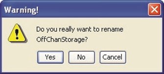A warning message (Figure 6.21) appears when you save the new name,
asking you to

confirm that you

want to rename the Off-Channel Storage Area project.

Figure 6.21 Warning Message when

Renaming Off-Channel

Storage Area

6.5.3 Removing an Off-Channel Storage Area from a Configuration

To remove an Off-Channel Storage Area from the current Configuration:

Select the Off-Channel Storage Tool and right-click on the Off-Channel Storage Area.
From the shortcut menu, select Remove from Configuration. This command removes the Off-Channel Storage project from the Configuration that is currently displayed in the Configuration box on the toolbar. The Confirm Removal dialog box will appear.

You can also remove an Off-Channel Storage Area from a Configuration by accessing the Configuration Editor and manually removing the project from the Projects tab using the Project Selector.

6.5.4 Deleting an Off-Channel Storage Area

To delete an Off-Channel Storage Area from the watershed:

Select the Off-Channel Storage Tool and right-click on the Off-Channel Storage Area.
From the shortcut menu, select Delete Off-Channel Storage. This command removes the Off-Channel Storage Area project and all data associated with it from the watershed. You will be asked to confirm a deletion before the Off-Channel Storage Area project is removed. Again, if you choose to delete the project, remember that deleting it may affect one or more of the configurations that recognize the Off-Channel Storage Area project.

6.5.5 Adding Configuration Notes for an Off-Channel Storage Area

To add Configuration Notes for an Off-Channel Storage Area:

Select the Off-Channel Storage Tool and right-click on the Off-Channel Storage Area.
From the shortcut menu, select Configuration Notes. This command opens a dialog box for entering text information about an Off-Channel Storage Area project that is specific to the configuration (Figure 6.22).

Figure 6.22 Configuration Notes for Off-Channel Storage

6.6 Creating "Other" Projects

To add "Other" Projects to the watershed:

Select the Other Project Tool .
Hold down the CTRL key and single click in the location where you want the other project to appear.

The Other Projects symbol will appear in the map display. Note that Other Projects are not yet implemented in ResSim's computations.

6.6.1 Editing "Other" Project Data

To edit "Other" Projects Data:

Select the Other Project Tool and right-click on the "Other" Project.
Select Edit Other Project. The Other Project Properties editor opens, as shown in Figure 6.23.

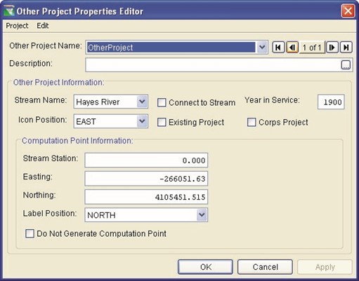
Figure 6.23 Other Project Properties Editor

The Other Project Properties editor allows you to define the spatial location (Coordinates), and contains basic configuration data, such as whether the project is an Existing Project, a Corps Project, the Label Position, the Stream Name, and the Year in Service (as previously described in Section 6.1.1).

Two options are unique to the Other Project Editor:

Connect to Stream checkbox allows you to associate the project with a particular stream in case it might be used with a supplemental model.
Do Not Generate Computation Point checkbox determines whether or not ResSim will automatically generate a Computation Point at the location specified in the Coordinates box.

6.6.2 Renaming "Other" Projects

To rename an "Other" Project:

Select the Other Project Tool and right-click on the Other Project.
From the shortcut menu, select Rename Other Project. This command opens a dialog box that allows you to rename the Other Project. If you choose to rename the project, remember that changing the project name may affect one or more of the configurations that recognize the Other Project.
A warning message
(Figure 6.24) appears when
you save the
new name, asking you to Figure 6.24 Warning Message when confirm that Renaming "Other" Project you want to rename the project.

6.6.3 Removing "Other" Projects from a Configuration

To remove an "Other" Project from the current Configuration:

Select the Other Project Tool and right-click on the Other Project.
From the shortcut menu, select Remove from Configuration. This command removes the Other Project from the
Configuration that is currently displayed in the Configuration box on the toolbar. The Confirm Removal dialog box appears.

You can also remove an Other Project from a Configuration by accessing the Configuration Editor and manually removing it from the Projects tab using the Project Selector.

6.6.4 Deleting "Other" Projects

To delete an "Other" Project from the watershed:

Select the Other Project Tool and right-click on the Other Project.
From the shortcut menu, select Delete Other Project. This command removes the Other Project and all data associated with it from the watershed. You will be asked to confirm a deletion before the Other Project is removed. Again, if you choose to delete the Other Project, remember that deleting it may affect one or more of the configurations that recognize the Other Project.

6.6.5 Adding Configuration Notes for "Other" Projects

To add Configuration Notes for an "Other" Project:

Select the Other Project Tool and right-click on the Other Project.
From the shortcut menu, select Configuration Notes. This command opens a dialog box (Figure 6.25) for entering text information about an Other Project that is specific to the configuration.

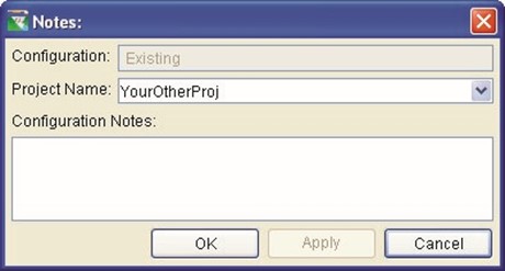
Figure 6.25 Configuration Notes for "Other" Projects

Configuring Project Display Properties

You can configure the appearance of Reservoirs, Levees, Diversions, and

Computation Points in the Study Layer of your watershed using the Study Properties Editor. See Chapter 4, Section 4.4.1, "Study Layer

Properties" for information on how to change Project display properties.

Defining Computation Points

The Computation Point set contains all locations where time-series information is to be computed. ResSim automatically generates Computation Points for the watershed based on Project, Stream Alignment, and Impact Area placement.

To add a Computation Point:

Lock the configuration.
Select the Computation Point Tool .
Hold down the CTRL key and click in the desired location.

The new Computation Point will appear in the map display. By default,

Computation Points snap to the stream alignment. If you prefer that the

Computation Point not snap to the stream alignment, de-select the Snap to Stream Alignment check box in the Computation Point Editor, described below.

6.8.1 Editing Computation Point Data

Use the Computation Point Editor to edit a Computation Point:

Lock the configuration.
Select the Computation Point Tool .
Right-click on the Computation Point to access the shortcut menu.
Select Edit Computation Point. The Computation Point Editor (Figure 6.26) will appear.

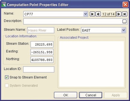
Figure 6.26 Computation Point Editor

The Computation Point Editor displays the information associated with a Computation Point and allows you to edit its location information.

Computation Point Name:

The Computation Point Editor displays the name of the Computation

Point you have selected (in the list along with all available

Computation Points in the watershed). Also, left and right arrows (navigator buttons) allow you to click through the Computation Points in the watershed.

Description:

To edit the Description of the Computation Point, you can type into the text area or click the button to access the Enter Description dialog box.

Stream Name:

The stream name automatically appears in the Stream Name box. In the case of a Computation Point situated at a confluence of two streams, you need to verify that the Computation Point resides on the appropriate stream.

Label Position: ResSim automatically positions the text label for a Computation Point where it is least likely to overlap other labels. However, you can move the position of the layer by selecting a position from the Label Position list.

Location Information:

Stream Station: The Stream Station field displays the location of the computation point along the stream element.
Easting / Northing: ResSim automatically fills in the coordinate information. You may type in new coordinates to relocate the Computation Point on the map display.

Location ID:

Optionally, you can enter a Location ID to reference the Computation Point to a ResSim ID.

Snap to Stream Alignment:

By selecting the Snap to Stream Alignment check box, you can place a Computation Point at any location and it will snap to the alignment. After a Computation Point is snapped on the stream alignment, only the Stream Station can be edited. ResSim automatically displays the Stream Name and Stream Stationing and Coordinates.

System Generated:

ResSim automatically generates Computation Points for the watershed based on Project placement. The System Generated checkbox is selected if the Computation Point has been system generated.

6.8.2 Renaming a Computation Point and Editing the Description

To rename a Computation Point or edit its description:

Lock the configuration.
Select the Computation Point Tool and right-click on the Computation Point.
Select Rename Computation Point.
Use the Rename dialog box (Figure 6.27) to edit the name and description. Click the button to access the Enter Description dialog box for longer descriptions.

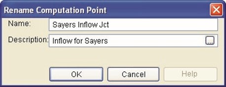
Figure 6.27 Rename Computation Point

6.8.3 Deleting a Computation Point

To delete a Computation Point:

Lock the configuration.
Select the Computation Point Tool and right-click on the Computation Point.
Select Delete Computation Point from the shortcut menu.

The Confirm Deletion dialog box will appear (Figure 6.28).

Click Yes to confirm the deletion.

Figure 6.28 Confirm Deletion of Computation Point

6.9 Working with Time-Series Icons

Time-Series Icons are not necessary for ResSim simulations. However, as part of watershed setup, you may need to configure them for other applications in the modeling software suite.

You can use Time-Series Icons to represent the locations of gages or Time-Series locations. Typically used in CWMS, they can be linked to data from either the Oracle Database or from a DSS file. The complete inventory of Time-Series Icons is viewable in the Watershed Setup Module. Figure 6.29 shows examples of the icons you can configure in the Watershed Setup Module.

Icons

Refer to the CWMS User's Manual (HEC, 2010) for additional information about Time-Series Icons.

Chapter 7

Creating Watershed Configurations

Table of Contents

Section Page

7 CREATING WATERSHED CONFIGURATIONS .................................................... 7-1

7.1 ADDING WATERSHED CONFIGURATIONS ...........................................................7 -1

7.2 ADDING AND REMOVING PROJECTS FROM CONFIGURATIONS ............................. 7-3

7.2.1 ADDING PROJECTS TO A CONFIGURATION ............................................. 7-4 7.2.2 REMOVING PROJECTS FROM A CONFIGURATION .................................... 7-4

7.3 ADDING PROJECT NOTES TO A CONFIGURATION ................................................ 7-5 7.4 MAKING A COPY OF A CONFIGURATION ............................................................. 7-5 7.5 DELETING A CONFIGURATION ...........................................................................7 -6 7.6 SAVING CONFIGURATION DATA.........................................................................7 -6 7.7 LISTING CONFIGURATIONS ...............................................................................7 -6

List of Figures

Figure Number Page

FIGURE 7.1 CONFIGURATION EDITOR ............................................................................7 -1 FIGURE 7.2 CREATE A NEW CONFIGURATION ................................................................7 -2 FIGURE 7.3 CALENDAR TOOL .......................................................................................7 -2

FIGURE 7.4 CONFIGURATION EDITOR – EDIT PROJECT LIST OPTION FROM

PROJECTS MENU ..................................................................................7 -3

FIGURE 7.5	PROJECT SELECTOR ..................................................................................7 -4
FIGURE 7.6	PROJECT NOTES EDITOR ...........................................................................7 -5
FIGURE 7.7	CONFIGURATION MENU, SAVE AS... ............................................................7 -5
FIGURE 7.8	CONFIRM DELETE OF A CONFIGURATION ..................................................... 7-6
FIGURE 7.9	LIST OF CONFIGURATIONS REPORT .............................................................7 -7

7-i

7-ii

Chapter 7

Creating Watershed Configurations

Once you have added all of the Projects and Computation Points needed for the watershed, you will need to create one or more Configurations. A Configuration is a specific physical arrangement of projects and computation points that will be modeled for the study of the watershed. Watershed Configurations are defined within the Watershed Setup Module.

ResSim provides enough flexibility to create Configurations for use in both real-time and planning contexts. ResSim creates a "superset" of all configurations (named Study) that contains all of the projects and computation points defined for the watershed. Additional Configurations you create reflect particular watershed conditions. For example, you might create Configurations for Existing Condition and Future Condition – 2030.

When you create additional Configurations, you can associate projects with specific Configurations, or add and remove them from the list of projects associated with a particular Configuration. You make

Configuration associations with Alternatives, as described in Chapter 13.

7.1 Adding Watershed Configurations

Watershed Configurations are added and edited within the Watershed Setup Module. To add a Configuration:

Lock the Configuration.
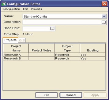From the Watershed menu, click
Configuration
Editor. The
Configuration
Editor
(Figure 7.1) will open.

Figure 7.1 Configuration Editor

In the Configuration menu, click New. The Create a New Configuration dialog box (Figure 7.2) will open.

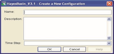
Figure 7.2 Create a New Configuration 4. Enter the Name (required) and Description (optional).

The Configuration Time Step is used when ResSim is operated as part of the Corps Water Management System (CWMS) software package, but it is also required even when using ResSim as standalone software. From the Time Step list, select a computation time step interval for the configuration.
Click OK to close the Create a New Configuration dialog box.
The name of the new configuration will appear in the Name list of the Configuration Editor, along with its defined Time Step.
Any project flagged as an Existing project (Chapter 6, Section 6.1.1), before you defined the new Configuration, will automatically be included in the table. To add projects (that are not flagged as Existing) to the configuration refer to Sections 7.2 and 7.2.1.
Once you have created the new Configuration, you can also optionally associate a Date with the Configuration. The Base Date field is used by some HEC applications (e.g., HEC-FIA), particularly in a planning context. You can either directly type the date into the field in the appropriate format (e.g., 01Feb2002), or use the Calendar Tool (Figure 7.3).
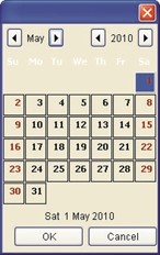To use the Calendar tool:

In the Configuration Editor, click on the button to the right of the Base Date field. The Calendar Tool will appear.
Select the month and year by clicking the left and right arrow buttons to navigate backwards and forwards. Select the day by clicking on the

appropriate day button. Figure 7.3 Calendar

Click OK to close the Calendar tool. Tool

When you are done creating the new
Configuration, Click OK to close the Configuration Editor.

7.2 Adding and Removing Projects from Configurations

As you set up your watershed and manage it over time, you may need to add new Projects to, or remove Projects from, Configurations you have created. To do this:

Select the Configuration you want to edit from the Configurations list on the toolbar.
Lock the Configuration.
Open the Configuration Editor from the Watershed menu.
From the Projects menu, select Edit Project List, as shown in Figure 7.4.

Figure 7.4 Configuration Editor – Edit Project List Option from Projects Menu

The Project Selector dialog box (Figure 7.5) will open. The Project Selector displays the Configuration name and description for reference. The left pane contains all Available Projects not already associated with the Configuration (in this example, two projects, Channel and ChannelMod). The Projects in Configuration pane on the right lists all Projects currently associated with the Configuration. Between the two panes are four buttons that enable you to add and remove projects of the Configuration by moving Projects from one pane to the other.

Figure 7.5 Project Selector

7.2.1 Adding Projects to a Configuration

To add Projects to an existing Configuration:

To add individual Projects, click on the Project's name in the Available Projects list (Figure 7.5) to select it, and then click the Add button to move it to the Projects in Configuration list.
To add all of the Available Projects to a Configuration, click the Add All button.
Click OK to save your changes and close the Project Selector dialog box.

7.2.2 Removing Projects from a Configuration

To remove Projects from an existing Configuration:

To remove individual Projects, click on the Project's name in the Projects in Configuration list (Figure 7.5) to select it, and then click the Remove button to move it to the Available Projects list.
To remove all of the Projects in Configuration from a Configuration, click the Remove All button.
Click OK to save your changes and close the Project Selector dialog box.

7.3 Adding Project Notes to a Configuration

Project notes within a Configuration are any comments that pertain specifically to a project in a particular Configuration. To Add or Edit project notes within a Configuration:

Select a project row in the Configuration Editor. If you do not select a project in the Configuration Editor before selecting the Project Notes menu item, you are alerted to select a project from the list.
Choose Project Notes from the Edit menu. The Project Notes dialog opens (Figure 7.6).

Figure 7.6 Project Notes Editor

When the Configuration Notes dialog opens, enter any Configuration-specific notes as needed.
Click OK to close the Configuration Notes dialog box.

7.4 Making a Copy of a Configuration

Sometimes you might want to make an exact copy of an existing configuration and then make some changes to it so you have a different configuration. To make a copy of a configuration:

On the Configuration Editor (Figure 7.1), from the Name list, select a configuration that you wish to copy.
From the Configuration menu, click Save As..., and the Save As. dialog box (Figure 7.7) opens.

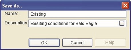
Figure 7.7 Configuration Menu, Save As...

The Name box contains the name of the selected configuration. Enter a new name in the Name box, and replace the description in the Description box.
Click OK to close the Save As dialog box. In the Name list on the Configuration Editor the new configuration is included.

7.5 Deleting a Configuration

To delete a configuration:

On the Configuration Editor (Figure 7.1), from the Name list, select the Configuration that you want to delete.
From the Configuration menu, select Delete.
A warning message (Figure 7.8) will open asking you whether you really want to delete the selected configuration. Click Yes, the warning message will close and the configuration name will no longer appear in the Name list on the Configuration Editor.

Figure 7.8 Confirm Delete of a Configuration

Saving Configuration Data

To save the data you have entered for a Configuration, from the

Watershed menu, click Save Configuration. This command will cause the program to save all configuration specific data.

Listing Configurations

Once you have all of your configurations entered, you might like to review the configurations in your watershed. From the Watershed Setup Module there is a report that contains this information.

To view the List of All Configurations:

You must be in the Watershed Setup Module. On the Module list, click Watershed Setup.
From the Reports menu, choose List of All Configurations, and the List of Configurations dialog box (Figure 7.9) will open.

Figure 7.9 List of Configurations Report

This report provides a list of configurations that have been input for the watershed. The list includes the Name and Description, along with the Time Step and Base Date (if entered) for each Configuration.
From the File menu, you can send the report to a printer, or you can export the report to an ASCII file. See Appendix F, Section F.4 for more details about printing and exporting tabulated data.
Click Close to close the List of Configurations report.

Chapter 8 Developing a Reservoir Network

Chapter 8

Developing a Reservoir Network

Table of Contents

Section Page

8 DEVELOPING A RESERVOIR NETWORK ............................................................ 8-1

8.1 RECOGNIZING RESERVOIR NETWORK SCREEN COMPONENTS ............................ 8-2

8.1.1 MENU BAR........................................................................................... 8-3 8.1.2 NETWORK, CONFIGURATION, AND LOCK/UNLOCK ................................... 8-5 8.1.3 MAP (MOUSE) TOOLS ........................................................................... 8-5 8.1.4 DISPLAY AREA ..................................................................................... 8-6

8.2 DEFINING A RESERVOIR NETWORK ................................................................... 8-7

8.2.1 CREATING A NEW RESERVOIR NETWORK .............................................. 8-7 8.2.2 OPENING AN EXISTING RESERVOIR NETWORK ....................................... 8-8 8.2.3 IMPORTING A RESERVOIR NETWORK ..................................................... 8-9 New

8.3 MAKING THE NETWORK EDITABLE ................................................................... 8-12 8.4 ADDING ROUTING REACHES ........................................................................... 8-12

8.4.1 DRAWING ROUTING REACHES............................................................. 8-12 8.4.2 RENAMING ROUTING REACHES ........................................................... 8-13 8.4.3 DELETING ROUTING REACHES ............................................................ 8-14

8.5 VIEWING NETWORK REPORTS ........................................................................ 8-14

8.5.1 VIEWING THE RESERVOIR LIST ............................................................ 8-14 8.5.2 VIEWING THE REACH LIST ................................................................... 8-15 8.5.3 VIEWING THE JUNCTION LIST .............................................................. 8-15 8.5.4 VIEWING THE DIVERSION LIST ............................................................. 8-16 8.5.5 VIEWING ADVANCED REPORTS ........................................................... 8-17

8.6 UPDATING A RESERVOIR NETWORK ................................................................ 8-19

8-i

List of Figures

Figure Page Number

FIGURE 8.1 RESERVOIR NETWORK MODULE MAIN WINDOW ............................................ 8-2

FIGURE 8.2 FILE MENU ..................................................................................................8 -3 FIGURE 8.3 EDIT MENU ................................................................................................. 8-3 FIGURE 8.4 VIEW MENU ................................................................................................8 -3

FIGURE 8.5 NETWORK MENU .........................................................................................8 -4 FIGURE 8.6 ALTERNATIVE MENU ....................................................................................8 -4 FIGURE 8.7 REPORTS MENU ..........................................................................................8 -4 FIGURE 8.8 TOOLS MENU ..............................................................................................8 -4 FIGURE 8.9 HELP MENU ................................................................................................8 -4

FIGURE 8.10 NETWORK, CONFIGURATION, AND LOCK/UNLOCK ICON ................................ 8-5 FIGURE 8.11 CREATE NEW RESERVOIR NETWORK ..........................................................8 -7 FIGURE 8.12 OPEN RESERVOIR NETWORK .....................................................................8 -8

FIGURE 8.13 IMPORT NETWORK WIZARD – STEP 1 OF 6

New

SELECT WATERSHED FROM WHICH TO IMPORT ...................................... 8-9

FIGURE 8.14 IMPORT NETWORK WIZARD – STEP 2 OF 6

SELECT NETWORK FROM WHICH TO IMPORT .......................................... 8-9 New

FIGURE 8.15 IMPORT NETWORK WIZARD – STEP 3 OF 6

DEFINE NEW NETWORK NAME AND DESCRIPTION ................................ 8-10^New

FIGURE 8.16 IMPORT NETWORK WIZARD – STEP 4 OF 6

ASSIGN STREAM NAMES .................................................................... 8-10 ^New

FIGURE 8.17 IMPORT NETWORK WIZARD – STEP 5 OF 6

New

(RESOLVE NETWORK COMPUTATION POINTS) ..................................... 8-11 FIGURE 8.18 IMPORT NETWORK WIZARD – STEP 6 OF 6 (IMPORT SUMMARY) .................. 8-11 ^New

FIGURE 8.19 CONTINUE WITH IMPORT .......................................................................... 8-12 _NewFIGURE 8.20 RENAME REACH ...................................................................................... 8-13 FIGURE 8.21 CONFIRM DELETE OF REACH.................................................................... 8-14 FIGURE 8.22 RESERVOIR NETWORK REPORTS: RESERVOIR LIST .................................. 8-14 FIGURE 8.23 RESERVOIR NETWORK REPORTS: REACH LIST ......................................... 8-15 FIGURE 8.24 RESERVOIR NETWORK REPORTS: JUNCTION LIST ..................................... 8-15 FIGURE 8.25 RESERVOIR NETWORK REPORTS: DIVERSION LIST ................................... 8-16

FIGURE 8.26 RESERVOIR NETWORK REPORTS: ADVANCED --

NETWORK CONNECTIVITY – "ALL" ELEMENTS" ..................................... 8-17

FIGURE 8.27 RESERVOIR NETWORK REPORTS: ADVANCED --

NETWORK CONNECTIVITY – "SELECTED" ELEMENTS" ........................... 8-18 FIGURE 8.28 RESERVOIR NETWORK REPORTS: ADVANCED -- NODE LIST ...................... 8-19

FIGURE 8.29 WATERSHED SETUP MODULE - WATERSHED MENU:

SAVE CONFIGURATION BEFORE UPDATING NETWORK ............................ 8-20

FIGURE 8.30 RESERVOIR NETWORK MODULE - NETWORK MENU:

UPDATE NETWORK FROM CONFIGURATION ........................................... 8-20

8-ii

Chapter 8 Developing a Reservoir Network

Chapter 8

Developing a Reservoir Network

A reservoir network represents a collection of watershed elements connected by routing reaches. Elements created in the Watershed Setup Module belong to specific watershed configurations, and when you create a reservoir network, it references one of those configurations.

The computation points defined for a configuration in the Watershed Setup Module automatically become junctions in the Reservoir Network Module. Your primary task in developing a reservoir network is to connect the junctions with routing reaches between junctions.

This chapter provides an overview of the Reservoir Network Module's screen components and describes the processes for creating a new reservoir network, opening an existing reservoir network, making a network editable, and adding routing reaches. ResSim also allows you to add additional elements to a reservoir network.

After you have established your reservoir network connectivity, you will need to edit Junction, Reach, and Diversion data (Chapter 9), define and edit the Physical components of Reservoirs in your network (Chapter 10), define Reservoir Operations data (Chapter 11), define Reservoir Systems (Chapter 12), and define Alternatives (Chapter 13). These steps will prepare your reservoir network to run Simulations (Chapter 14).

8.1 Recognizing Reservoir Network Screen Components

The Reservoir Network Module (Figure 8.1) provides the tools you will need to develop the connectivity of your reservoir network as well as enter and edit physical and operations data. What follows is a discussion of the components and features of the Reservoir Network Module.

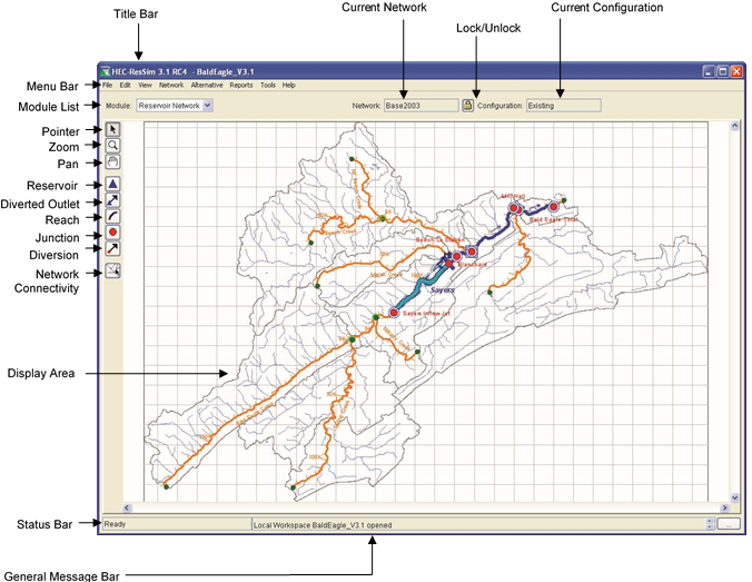
Figure 8.1 Reservoir Network Module Main Window

8.1.1 Menu Bar

The following is an overview of the Reservoir Network Module's Menu Bar tools, which allow you to create and edit the connectivity of your reservoir network. The tools specific to this module will be described in more detail in the context of particular tasks later in this chapter.

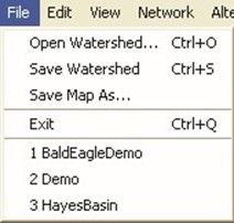The File menu (Figure 8.2) allows you to Open an existing watershed, Save a watershed, Save the Display Area (Map), and Exit ResSim. Your most-recently-used watersheds are listed at the bottom of the File menu.

Figure 8.2 File Menu

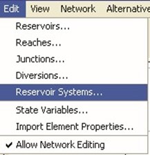The Edit menu (Figure 8.3) provides access to the ResSim editors for Reservoirs, Reaches, Junctions, Diversions, and Reservoir Systems. Access to the editor for State Variables and the steps to Import Element Properties are available. You must select the Allow Network Editing option to access the editors.

Figure 8.3 Edit Menu

In the View menu (Figure 8.4) select Zoom to All to restore your watershed map view to full size. Layers opens the Layer Selector dialog box. Unit System allows you to customize the display (view) settings for your watershed. If a dialog or editor window is open but

inactive, Restore Windows brings the dialog

or editor window to the front as the active

window. The Grid Lines option allows for Figure 8.4 View Menu turning on or off the grid lines in the map region.

The Network menu (Figure 8.5) is unique to the Reservoir Network Module. It allows you to create a New network, Open an existing network, Edit the description of an opened network, Save a network or Save As a new network, or Rename a network. You can also Update Network from Configuration, Import Network, and Delete Networks.

Figure 8.5 Network Menu

access to the Alternative Editor.

Figure 8.6

Alternative Menu

The Alternative menu (Figure 8.6), also

available in the Simulation Module, provides

the Node List reports.

Figure 8.7

Reports Menu

As in the other modules, the Tools menu (Figure

the information written to the ResSim.log file. Information provides details about client, user, and watershed settings as well as server and system properties.

Figure 8.8 Tools

Menu

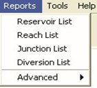
The Reports menu (Figure 8.7) provides access to the Reservoir List, Reach List, Junction List, and Diversion List. Also, two Advanced reports are available: the Network Connectivity

(for All Elements or for Selected Elements) and

8.8) provides access to HEC-DSSVue and to

Scripts. Options allows you specify Model

Directories, Compute Display, Debug Levels, General information (including whether to show a confirmation when exiting the program and whether to reload last watershed at startup of

program), and Fonts. Console Output displays

In the Help menu (Figure 8.9) the About HEC-ResSim command displays information about the version of ResSim. Also, from this menu you can access user documentation and Install Example

Watersheds (after you define a watershed

location as described in Section 3.3.1). Figure 8.9 Help Menu

8.1.2 Network, Configuration, and Lock/Unlock

In the Reservoir Network Module, your current Reservoir Network and Configuration, along with the Lock/Unlock icon , are displayed below the Menu Bar and to the right of the Module List, as shown in Figure 8.10.

Figure 8.10 Network, Configuration, and Lock/Unlock Icon

The Configuration indicates which configuration the current Network is based on. As will be described in Section 8.2, you select the Configuration when you create the Network (using the Network menu).

The Lock/Unlock icon indicates whether or not the Network is locked and available for editing. You can lock and unlock the Network by clicking on the icon or by selecting or deselecting Allow Editing in the Edit menu.

8.1.3 Map (Mouse) Tools

The Map (Mouse) Tools, which appear in the toolbar on the left side of the ResSim screen, allow you to interact with objects in the map display. The Reservoir Network Module has three standard Map Tools and five network connectivity tools that allow you to establish the connectivity of your reservoir network.

Pointer Tool

Right-click with the Pointer Tool to select and access a shortcut menu for any schematic element within your map display. The Pointer Tool is available in all ResSim modules.

Zoom Tool

The Zoom Tool allows you to zoom in and out of the display area in all modules. To zoom in, hold the left mouse button down and outline the area you want to enlarge. To zoom out, click the right mouse button. Zooming out using the right click button zooms out by a factor of two, positioning the clicked location at the center of the screen. The Zoom Tool is available in all ResSim modules.

Pan Tool

After you have zoomed in with the Zoom Tool, you can use the Pan Tool to view watershed areas that fall outside of the ResSim window borders. The Pan Tool is available in all ResSim modules.

Reservoir Tool

With the Reservoir Tool, you can add reservoirs to your reservoir

network. You can also edit reservoir properties, rename, and delete reservoirs using commands in the shortcut menu.

Diverted Outlet Tool

The Diverted Outlet Tool allows you to create a diverted outlet from a reservoir in your network. The shortcut menu for this tool provides access to the Reservoir Editor and also allows you to rename and delete a diverted outlet.

Reach Tool

Use the Reach Tool to draw routing reaches (from upstream to downstream) to connect the junctions on the stream alignment. You can also edit reach properties, rename, break, and delete reaches using commands in the shortcut menu.

Junction Tool

The Junction Tool allows you to manually insert junctions in your reservoir network. The shortcut menu for this tool allows you to edit junction properties, rename and delete junctions.

Diversion Tool

With the Diversion Tool you can add diversions to your reservoir network. You can also edit diversion properties, rename, delete, and disconnect outflow of diversion reaches using commands in the shortcut menu.

Network Connectivity Tool

Using the Network Connectivity Tool you can click on any element in the map display area to see which elements are connected (connected elements will be highlighted). If you right-click on an element, you can choose to show the upstream or downstream connectivity.

8.1.4 Display Area

In the Reservoir Network Module, the display area contains the reservoir network connectivity you construct, along with the map layers, stream alignment, reservoirs and computation points you have established in the Watershed Setup Module for the current network's configuration. Any other time-series icons, projects, and impact areas you established in the Watershed Setup Module will not appear.

Using the Map (Mouse) Tools to access shortcut menus, you can open

data editors as well as rename and delete elements in your reservoir network directly from the display area.

8.2 Defining a Reservoir Network

With a stream alignment in place and one or more configurations defined, you can create a network of reservoirs and routing reaches. This process involves defining a new network and then adding routing reaches.

8.2.1 Creating a New Reservoir Network

When you create a new reservoir network, you are defining which elements will be included in your network by selecting the appropriate watershed configuration. Once you have created your network, you can add additional elements. Remember, however, that any additional elements you add will not be available for use in other networks. If you want the additional elements to be available for other networks, you will need to go back to the Watershed Setup Module and add the new elements to the appropriate configuration, then return to the Reservoir Network Module to create your reservoir network using the updated configuration (Section 8.6, "Updating a Reservoir Network").

To create a new reservoir network:

From the Network menu, select New. The Create New Reservoir Network dialog box will appear (Figure 8.11).

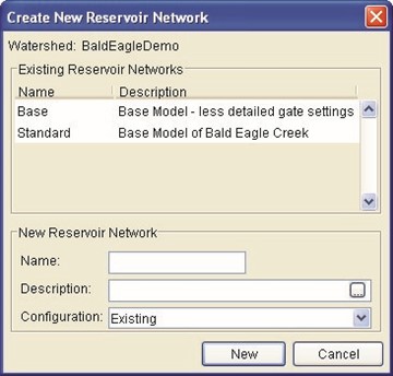
Figure 8.11 Create New Reservoir Network

Specify a Name for the network and enter a Description. You can click the button to access a larger text field for your description.
From the Configuration list, choose the configuration on which this network will be based.
Click New.

The Create New Reservoir Network dialog box will close, and you will see the name of your new network and its configuration displayed below the Menu Bar, to the right of the Module List (see Section 8.1.2 above).

In the display area, ResSim will automatically create the reservoirs and computation points that were part of the selected configuration as elements in the new Reservoir Network. Reservoirs transfer directly, whereas Computation points appear as Junctions.

8.2.2 Opening an Existing Reservoir Network

To open an existing Reservoir Network for editing:

From the Network menu, select Open. The Open Reservoir Network dialog box will appear (Figure 8.12).

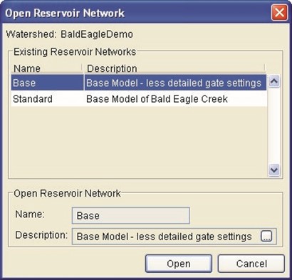
Figure 8.12 Open Reservoir Network

Select the Reservoir Network you want by clicking on it.
Click Open.

The Open Reservoir Network dialog box will close, and you will see the name of your network and its configuration displayed below the Menu Bar, to the right of the Module List (see Section 8.1.2 above).

8.2.3 Importing a Reservoir Network

To use the Import Network Wizard, perform the following steps:

From the Network menu in the Reservoir Network module, select Import Network…. The Import Network Wizard – Step 1 of 6 will appear (Figure 8.13). Select the Watershed Watershed that contains the network from which you would like to import the entire network physical and operational data. The box on the left side of the dialog contains names of Watershed Locations that have been specified as Model Directories. The box on the right side of the dialog contains all the watersheds that can be found in each Watershed Location.

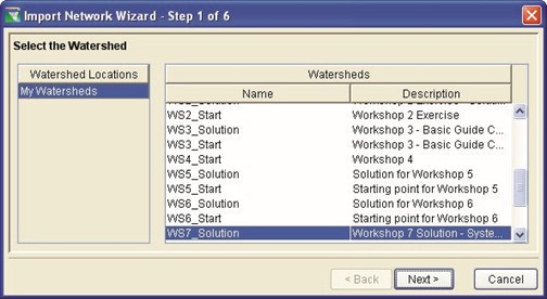
Figure 8.13 Import Network Wizard – Step 1 of 6

Select Watershed from which to Import

Select Next and Import Network Wizard - Step 2 of 6 will appear. Select the network from which you would like to import all elements by highlighting the Network Name (Figure 8.14).

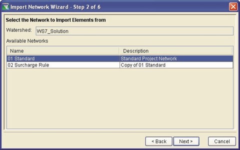
Figure 8.14 Import Network Wizard – Step 2 of 6

Select Network from which to Import

Next to continue and the Import Network Wizard – Step 3 of 6 will appear (Figure 8.15). Enter a New Reservoir Network Name and Description.

Figure 8.15 Import Network Wizard – Step 3 of 6

Define New Network Name and Description

Select Next to continue and the Import Network Wizard – Step 4 of 6 will appear (Figure 8.16). Assign Stream Names by dropdown menu one at a time, or at once by selecting the Assign Stream Names button. Care is required in determining the connection of the Imported Element to the Stream. If Imported Elements are associated with streams that are not connected, it is possible there will be erroneous downstream control rules added to upstream junctions.

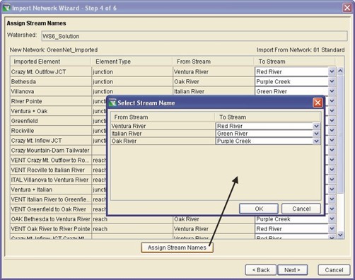
Figure 8.16 Import Network Wizard – Step 4 of 6

Assign Stream Names

Next to continue and the Import Network Wizard – Step

5 of 6 will appear (Figure 8.17). Assign the network elements to their corresponding watershed computation points by use of a drop-down menu for each imported element.

Figure 8.17 Import Network Wizard – Step 5 of 6

(Resolve Network Computation Points)

Select Next to continue and the Import Network Wizard – Step 6 of 6 will appear (Figure 8.18). Review all of the information in the import summary. Check to ensure that all physical and operational data was successfully imported by reviewing the Import Summary and by viewing the various network element editors in the Reservoir Network module.

Figure 8.18 Import Network Wizard – Step 6 of 6

(Import Summary)

Finish to carry out the Network import, or select Back to make changes in previous steps. If you are sure about the import, confirm by selecting Yes in the Continue with Import dialog box (Figure 8.19). Choosing No will return you to the Wizard's Step 6 of 6.

Figure 8.19 Continue with Import

Select the Close button to complete the process of Importing a Reservoir Network from one Watershed/Network into another.
1. Making the Network Editable

Before you can begin editing your reservoir network, you must ensure that the network is editable ("locked"). To do so, select Allow Network Editing from the Edit menu or click the Lock/Unlock button .

Adding Routing Reaches

Routing reaches are elements that establish the connectivity of the reservoir network schematic. By adding a routing reach between two junctions, you can connect the reservoir network so that water will transverse through the routing reach from upstream to downstream.

Drawing Routing Reaches

Routing Reaches are drawn from upstream to downstream. You connect two adjacent junctions (typically, computation points added to the network's Configuration in the Watershed Setup Module) by drawing a routing reach.

To draw routing reaches:

Select the Reach Tool .
Point to the upstream junction at the upstream end of the reach.
Hold down the CTRL key and click on the junction to start the upstream end of the reach.
Release the CTRL key and move the mouse pointer along the stream alignment and click on the downstream junction.

Routing reaches automatically conform to the stream alignment. You can connect routing reaches to existing junctions; otherwise, if you begin and/or end a reach elsewhere on the stream alignment, ResSim will create new junctions at both/either end of the reach.

ResSim will automatically constrain a new reach between existing junctions (e.g., will not allow a reach to be drawn past an existing junction). If the reach appears to draw past a junction, then the junction is not on the stream you think it's on. This can occur if the computation point (that the junction is based on) is not initially placed on the appropriate stream. To solve this situation, go back to the Watershed Setup Module and revise the location of the computation point (you may need to delete and recreate the computation point to be on the appropriate stream). After saving your watershed configuration, change to the Reservoir Network Module and select Update Network from Configuration from the Network menu. See Section 8.6, "Updating a Reservoir Network" for additional information for updating networks.

Additionally, you may not connect tributaries to the middle of a reach; tributaries must connect to a junction.

Renaming Routing Reaches

ResSim automatically names routing reaches according to the names of the upstream and downstream junctions. To rename a reach component:

Select the Reach Tool .
Right-click on the routing reach to be renamed.
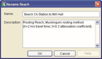Select Rename from the shortcut menu. The Rename Reach dialog box will appear (Figure 8.20), allowing you to type in a new name.
Type in the new

name and optional

description. Figure 8.20 Rename Reach

Click OK to close the Rename Reach dialog box.

The new name will now appear as a label in the map display.

Deleting Routing Reaches

To delete routing reaches:

Select the Reach Tool .
Right-click on the routing reach to be deleted.
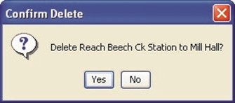Select Delete from the shortcut menu. A Confirm Delete dialog box will appear (Figure 8.21).
Click Yes if you are

sure about the Figure 8.21 Confirm Delete of Reach deletion.

The deleted routing reach will no longer appear in the map display.

Viewing Network Reports

In the Reservoir Network Module, the Reports menu allows you to access summary reports pertinent to the elements in your network. These reports summarize your reservoirs, routing reaches, junctions, and diversions. In addition, advanced reports of your network connectivity are also available. The Report contents can be "sorted" alphabetically by clicking on a column header in the report. Also, when an element is selected in the report listing, that element is highlighted in the Map Display area.

Viewing the Reservoir List

The Reservoir List (Figure 8.22) displays the names and descriptions of all reservoirs in your network. Additionally, the number of reservoirs is listed in the bottom right corner. For information about printing and exporting options available from the report's Report menu, see Appendix F. The Edit menu provides access to the Reservoir Editor (after selecting a reservoir in the list and then selecting Edit from the Edit menu).

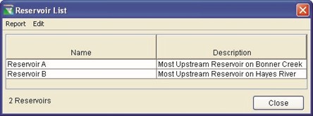
Figure 8.22 Reservoir Network Reports: Reservoir List

Viewing the Reach List

The Reach List (Figure 8.23) displays the names, descriptions, routing method, and losses of all reaches in your network. For information about printing and exporting options available from the report's Report menu, see Appendix F. The Edit menu provides access to the Reach Editor (after selecting a reach in the list and selecting Edit from the Edit menu).

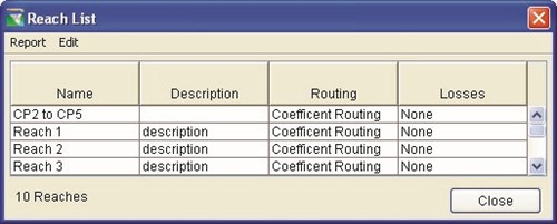
Figure 8.23 Reservoir Network Reports: Reach List

Viewing the Junction List

The Junction List (Figure 8.24) displays the names and descriptions of all junctions in your network. For information about printing and exporting options available from the report's Report menu, see Appendix F. The Edit menu provides access to the Junction Editor (after selecting a junction in the list and selecting Edit from the Edit menu).

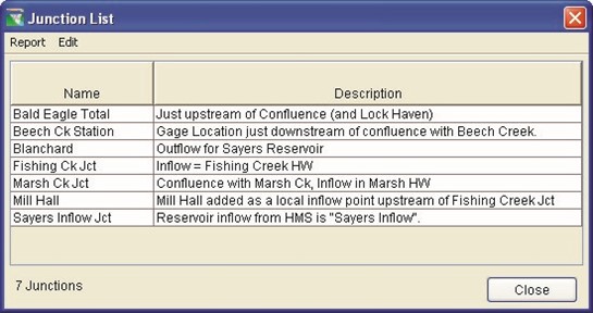
Figure 8.24 Reservoir Network Reports: Junction List

Viewing the Diversion List

The Diversion List (Figure 8.25) displays the names, descriptions, and method of all diversions in your network. For information about printing and exporting options available from the report's Report menu, see Appendix F. The Edit menu provides access to the Diversion Editor (after selecting a diversion in the list and selecting Edit from the Edit menu).

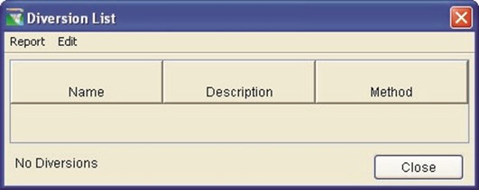
Figure 8.25 Reservoir Network Reports: Diversion List

Viewing Advanced Reports

Two Advanced Reports are available from the Reports menu:

The first advanced report is the Network Connectivity summary. This report provides a connectivity summary of "all" or "selected" elements/nodes in your reservoir network. Details include Element/Node (the "type" of Element and associated Inflow and Outflow Nodes), ID, Name, Function/Upstream Element, and Parent/Downstream Element.

The All Elements connectivity report (Figure 8.26) is accessed from the Reports menu by selecting:
Advanced  Network Connectivity  All Elements

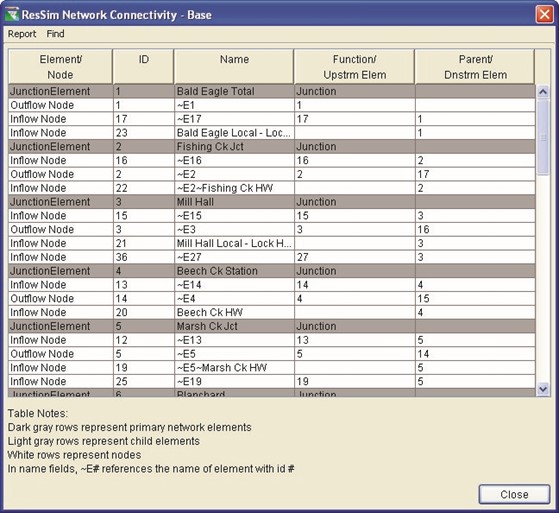
Figure 8.26 Reservoir Network Reports: Advanced --

Network Connectivity – "All" Elements"

For information about printing and exporting options available from the report's Report menu, see Appendix F. The Find menu allows you to find text strings within the report.

The Selected Elements connectivity report (Figure 8.27) is accessed by first selecting elements in the Map Display area by holding down the SHIFT key and clicking on the desired elements (performs multiple selections as indicated in the map shown in Figure 8.27). Then, from the Reports menu, select: Advanced  Network Connectivity  Selected Elements

Figure 8.27 Reservoir Network Reports: Advanced --

Network Connectivity – "Selected" Elements"

For information about printing and exporting options available from the report's Report menu, see Appendix F. The Find menu allows you to find text strings within the report.

The second advanced report is the Node List (Figure 8.28). This report provides a summary of all nodes in your reservoir network. Details include the Node ID, Name, Key String, Upstream Element, Downstream Element, Stream, Stream Station, and Stream Coordinate (i.e., a normalized position on the stream).

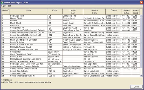
Figure 8.28 Reservoir Network Reports: Advanced -- Node List

For information about printing and exporting options available from the report's Report menu, see Appendix F. The Edit menu provides two options: Clean Network and Delete Node. These options can potentially damage a working network and should only be used when recommended by a ResSim technical expert.

8.6 Updating a Reservoir Network

In the Watershed Setup Module, if you make changes (e.g., add, delete, move or rename elements) to the watershed configuration your network is based on, you need to update your Reservoir Network to include those changes. First, in the Watershed Setup module, from the Watershed menu, select Save Configuration (Figure 8.29).

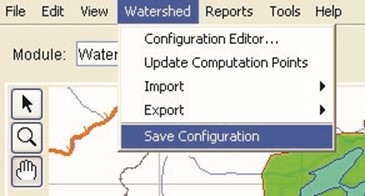
Figure 8.29 Watershed Setup Module - Watershed Menu: Save Configuration before Updating Network

Next, in the Reservoir Network module, with the network to be updated shown in the display area, select Update Network from Configuration from the Network menu (Figure 8.30).

Figure 8.30 Reservoir Network Module -

Network Menu: Update Network from Configuration

After the network has been updated from the revised Configuration, you should see the revisions reflected in the Map Display area.

You will need to update each Reservoir Network that is based on the revised Watershed Configuration.

ResSim User's Manual

Chapter 9

Editing Junction, Reach, and Diversion Data

Table of Contents

Section Page

9 EDITING JUNCTION, REACH, AND DIVERSION DATA ....................................... 9-1

9.1 EDITING JUNCTION PROPERTIES .......................................................................9 -1

9.1.1 JUNCTION EDITOR: INFO TAB ...............................................................9 -2 9.1.2 JUNCTION EDITOR: LOCAL FLOW TAB ................................................... 9-3 9.1.3 JUNCTION EDITOR: RATING CURVE TAB ................................................ 9-4 9.1.4 JUNCTION EDITOR: OBSERVED DATA TAB ............................................. 9-5

9.2 EDITING REACH PROPERTIES ...........................................................................9 -6

9.2.1 REACH EDITOR: ROUTING TAB .............................................................9 -7 9.2.2 REACH EDITOR: LOSSES TAB ............................................................. 9-18 9.2.3 REACH EDITOR: OBSERVED DATA TAB ............................................... 9-18

9.3 EDITING DIVERSION PROPERTIES ................................................................... 9-19

9.3.1 DIVERSION EDITOR: DIVERSION TAB ................................................... 9-20 9.3.2 DIVERSION EDITOR: ROUTING TAB ..................................................... 9-34 9.3.3 DIVERSION EDITOR: LOSSES TAB ....................................................... 9-34 9.3.4 DIVERSION EDITOR: OBSERVED DATA TAB ......................................... 9-35

9-i

List of Figures

Figure
Number	Page
FIGURE 9.1	JUNCTION EDITOR: INFO TAB .....................................................................9 -2
FIGURE 9.2	JUNCTION EDITOR: LOCAL FLOW TAB .........................................................9 -3
FIGURE 9.3	JUNCTION EDITOR: RATING CURVE TAB ..................................................... 9-4
FIGURE 9.4	JUNCTION EDITOR: OBSERVED DATA TAB ................................................... 9-5
FIGURE 9.5	REACH EDITOR: ROUTING TAB ................................................................... 9-6
FIGURE 9.6	REACH EDITOR: COEFFICIENT ROUTING METHOD ....................................... 9-7
FIGURE 9.7	REACH EDITOR: MUSKINGUM ROUTING METHOD ........................................ 9-8
FIGURE 9.8	REACH EDITOR: MUSKINGUM-CUNGE 8-PT CHANNEL ROUTING METHOD ...... 9-9
FIGURE 9.9	REACH EDITOR: MUSKINGUM-CUNGE PRISMATIC

CHANNEL ROUTING METHOD .............................................................. 9-11 FIGURE 9.10 REACH EDITOR: MODIFIED PULS ROUTING METHOD ................................ 9-13 FIGURE 9.11 REACH EDITOR: SSARR ROUTING METHOD ........................................... 9-14 FIGURE 9.12 REACH EDITOR: WORKING R&D ROUTING METHOD ................................ 9-16 FIGURE 9.13 REACH EDITOR: VARIABLE LAG & K METHOD .......................................... 9-17^New FIGURE 9.14 REACH EDITOR: LOSSES TAB ................................................................. 9-18 FIGURE 9.15 REACH EDITOR: OBSERVED DATA TAB ................................................... 9-19 FIGURE 9.16 DIVERSION EDITOR ................................................................................. 9-19

FIGURE 9.17 DIVERSION EDITOR: CONSTANT DIVERSION METHOD ............................... 9-21 FIGURE 9.18 DIVERSION EDITOR: MONTHLY VARYING DIVERSION METHOD .................. 9-22 FIGURE 9.19 DIVERSION EDITOR: SEASONAL DIVERSION METHOD ............................... 9-23 FIGURE 9.20 DIVERSION EDITOR: FUNCTION OF FLOW DIVERSION METHOD ................. 9-24 FIGURE 9.21 DIVERSION EDITOR: FUNCTION OF POOL ELEVATION DIVERSION METHOD 9-25 FIGURE 9.22 DIVERSION EDITOR: TIME-SERIES DIVERSION METHOD ............................ 9-26 FIGURE 9.23 DIVERSION EDITOR: FLEXIBLE DIVERSION RULE METHOD ........................ 9-27 FIGURE 9.24 DIVERSION EDITOR: FLEXIBLE DIVERSION RULE –

SELECT INDEPENDENT VARIABLE ....................................................... 9-27

FIGURE 9.25 DIVERSION EDITOR: FLEXIBLE DIVERSION--FUNCTION OF DATE ................ 9-28 FIGURE 9.26 HOUR OF DAY MULTIPLIER WITH DEFAULT VALUES OF 1.0

SPECIFIED FOR ENTIRE DAY .............................................................. 9-29

FIGURE 9.27 HOUR OF DAY MULTIPLIER WITH VALUES OF 1.5

SPECIFIED FOR PORTION OF DAY ....................................................... 9-29

FIGURE 9.28 DAY OF WEEK MULTIPLIER WITH DEFAULT FACTORS OF 1.0

SPECIFIED FOR EACH DAY OF THE WEEK ........................................... 9-30

FIGURE 9.29 DAY OF WEEK MULTIPLIER WITH FACTORS OF 0.0

SPECIFIED FOR SATURDAY AND SUNDAY ............................................ 9-30

FIGURE 9.30 DIVERSION EDITOR: FLEXIBLE DIVERSION--FUNCTION OF

DATE & TIME .................................................................................... 9-31

FIGURE 9.31 DIVERSION EDITOR: FLEXIBLE DIVERSION--FUNCTION OF

MODEL VARIABLE ............................................................................. 9-31

FIGURE 9.32 DIVERSION EDITOR: FLEXIBLE DIVERSION--FUNCTION OF

EXTERNAL VARIABLE ......................................................................... 9-32

FIGURE 9.33 DIVERSION EDITOR: FLEXIBLE DIVERSION--FUNCTION OF

STATE VARIABLE............................................................................... 9-33

FIGURE 9.34 TIME SERIES OPTIONS FOR MODEL, EXTERNAL, AND

STATE VARIABLE INDEPENDENT VARIABLES ........................................ 9-33 FIGURE 9.35 DIVERSION EDITOR: LOSSES TAB ........................................................... 9-34 FIGURE 9.36 DIVERSION EDITOR: OBSERVED DATA TAB .............................................. 9-35 9-ii

Chapter 9

Editing Junction, Reach, and Diversion Data

Once you have established the connectivity of your Reservoir Network (Chapter 8), you can define and edit the properties of elements in the network. You will need to specify parameters for all junctions, reaches, diversions, and reservoirs using ResSim's specialized editors. You will also need to edit the physical and operations data for reservoirs, as described in Chapters 10-11.

This chapter explains how to enter and edit data for junctions, reaches, and diversions. Refer to Chapter 8 for developing a Reservoir Network within the Reservoir Network Module.

9.1 Editing Junction Properties

To edit junction data, select the Junction Tool and right-click on a junction. From the shortcut menu, select Edit Junction Properties. The Junction Editor will open.

The Name field at the top of the editor contains a list of all of the junctions in your reservoir network, with the name of the selected junction displayed. You can access all of the junctions both from this list and by using the VCR-style buttons to navigate through the available junctions.

The Junction Editor has four tabs that allow you to edit junction information (Info), Local Flow, Rating Curve, and Observed Data, as described in the following sections.

9.1.1 Junction Editor: Info Tab

The Info tab (Figure 9.1) displays the Description, Stream Station,

Stream, and Tributaries you have defined within the Watershed Setup Module and during the process of creating your reservoir network within the Reservoir Network Module.

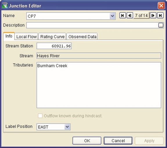
Figure 9.1 Junction Editor: Info Tab

The Stream and Tributaries fields are not editable, but you may revise the junction Description and Stream Station. If the historic outflow for a junction is available for the hindcast (lookback) period, then click on the Outflow known during hindcast box. An entry will appear in the time-series table that you will complete during the creation of an Alternative (Chapter 13).

You may also choose the position of the name label in your map display from the options in the Label Position field.

To edit properties for other junctions without exiting the Junction Editor, click the Apply button and then select another junction from the Name list or use the navigator buttons.

9.1.2 Junction Editor: Local Flow Tab

On the Local Flow tab (Figure 9.2) of the Junction Editor, you can input a Name and Factor in the table for each external flow entering the junction.

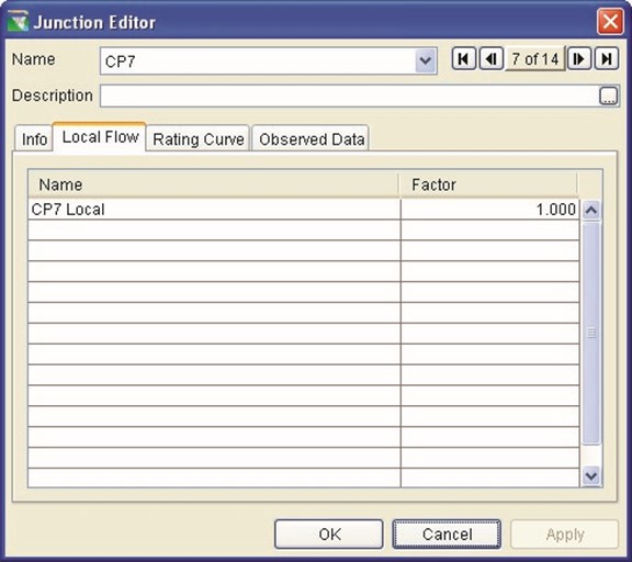
Figure 9.2 Junction Editor: Local Flow Tab

Name: The name you enter will appear during the Alternative definition to identify the local flow for time-series mapping (Chapter 13). This name CANNOT be the same as the Junction name.
Factor: The factor value is available to increase or decrease the local flow hydrographs. If you enter a value of 1.0, then the local flow will be equal to the hydrograph reference.

You must define flows for headwater junctions. Flows are optional at other junctions.

If you specify an entry on the Local Flow tab, then you will see a circle (i.e., a "halo") around the junction as a "visual reminder" to indicate which locations will receive local inflows.

To edit properties for other junctions without exiting the Junction Editor, click the Apply button and then select another junction from the Name list or use the navigator buttons.

9.1.3 Junction Editor: Rating Curve Tab

The Rating Curve tab (Figure 9.3) is optional. However, if you need stages calculated at a junction, you can enter Stage and Discharge values for the junction here. The mini-plot will reflect the values you enter and can be viewed in full size when you double-click on it.

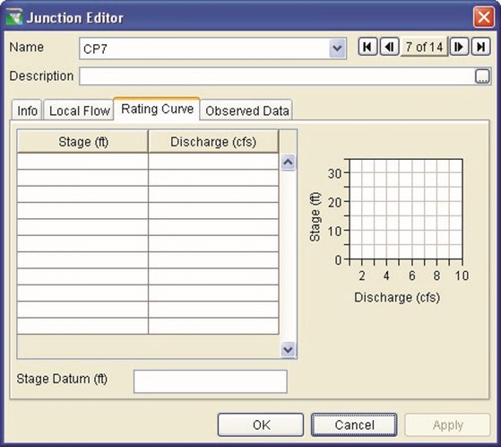
Figure 9.3 Junction Editor: Rating Curve Tab

Stage: Enter Stage values (in meters or feet) that correspond to the Discharge values.
Discharge: Enter Discharge (flow) values (in cms or cfs) that correspond to the Stage values.

To edit properties for other junctions without exiting the Junction Editor, click the Apply button and then select another junction from the Name list or use the navigator buttons.

9.1.4 Junction Editor: Observed Data Tab

Use the Observed Data tab (Figure 9.4) to indicate that observed data is available for comparison purposes. If the Observed box in the table is checked (as shown in Figure 9.4), then there will be a corresponding entry in the Observed Time-Series mapping table when you create an Alternative (Chapter 13).

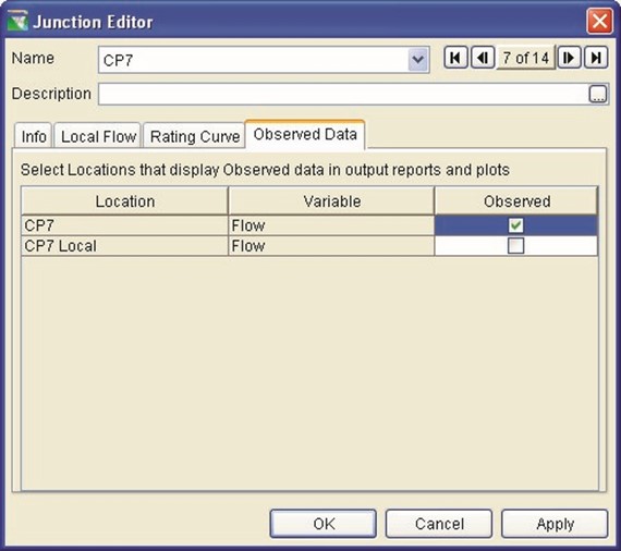
Figure 9.4 Junction Editor: Observed Data Tab

To edit properties for other junctions without exiting the Junction Editor, click the Apply button and then select another junction from the Name list or use the navigator buttons.

9.2 Editing Reach Properties

To edit routing reach data, select the Reach Tool and right-click on a routing reach. From the shortcut menu, select Edit Reach Properties. The Reach Editor will open (Figure 9.5).

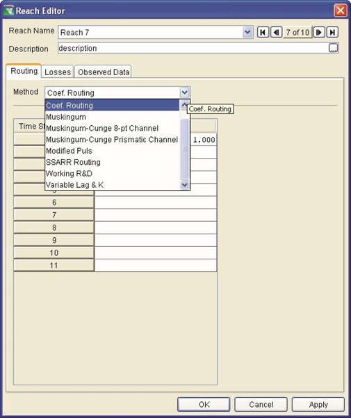
Figure 9.5 Reach Editor: Routing Tab

The Reach Name field at the top of the editor contains a list of all of the routing reaches in your reservoir network, with the name of the selected reach displayed. You can access all of the reaches from this list or by using the VCR-style buttons to navigate through the available reaches.

Below the Reach Name list is the Description of the current reach; this field is editable.

The Reach Editor has three tabs that allow you to edit Routing methods, Losses, and Observed Data, as described in the following sections.

9.2.1 Reach Editor: Routing Tab

The Reach Editor's Routing tab (as previously shown in Figure 9.5) allows you to choose from eight routing methods: Coefficient,

Muskingum, Muskingum-Cunge 8-pt Channel, Muskingum-Cunge Prismatic Channel, Modified Puls, SSARR, Working R&D Routing, and Variable Lag & K; each method with its own set of parameters. If there is no lag or translation of the hydrograph through the reach, you can select Null Routing. Select the routing method for the reach from the Method list. The appropriate fields for data entry will appear according to the method you have selected.

9.2.1.1 Coefficient Routing Method

For the Coefficient Routing method (Figure 9.6), you will need to enter coefficients for each time step of the routing extent. Each coefficient equates to the fraction of the flow entering the reach that will reach the downstream end at the end of each time step in the table. The values in the table must sum up to 1.

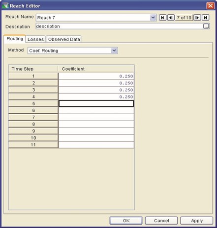
Figure 9.6 Reach Editor: Coefficient Routing Method

If you enter a 1 in the first row and leave the rest of the table blank, you have effectively described null or noroute routing. This means that 100% of the flow entering the reach instantaneously leaves the reach in that time step.

To edit another reach without exiting the Reach Editor, click the Apply button and then select another reach from the Name list or use the navigator buttons.

9.2.1.2 Muskingum Routing Method

The Muskingum routing method (Figure 9.7) requires you to enter values for Muskingum K (in hours) and Muskingum X. You will also need to specify the Number of Subreaches.

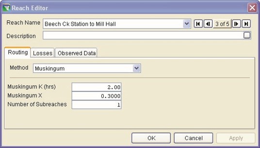
Figure 9.7 Reach Editor: Muskingum Routing Method

Muskingum K: Enter the number of hours (travel time) for the reach, i.e., how long it takes for a drop of water that enters the reach to exit the reach.
Muskingum X: Enter the attenuation coefficient (from 0.0 to 0.5). A value of 0.0 indicates maximum attenuation of the hydrograph through the routing reach. A value of 0.5 indicates a "direct translation" of the hydrograph through the reach.
Number of Subreaches: Number of steps (subreaches) applicable for the routing reach. This parameter should be approximately equal to travel time divided by the computation interval.

To edit another reach without exiting the Reach Editor, click the Apply button and then select another reach from the Name list or use the navigator buttons.

9.2.1.3 Muskingum-Cunge 8-pt Channel Routing Method

The Muskingum-Cunge 8-pt Channel routing method (Figure 9.8) uses a representative eight-point channel cross section to perform the Muskingum-Cunge hydrologic routing method. This method requires that you enter the Channel Length and Channel Slope, as well as eight Station and Elevation values to describe the cross section. The cross section displays in both a generalized illustration of a cross section and a mini-plot of the data you enter and can be viewed in full size when you double-click on it. Other parameters you will need to enter are Manning's n Values for the Left Overbank, Main Channel, and Right Overbank. The Default Reference Flow value is used to compute the celerity for the reach. The Routing Timestep Subintervals value can vary from 1 to 12.

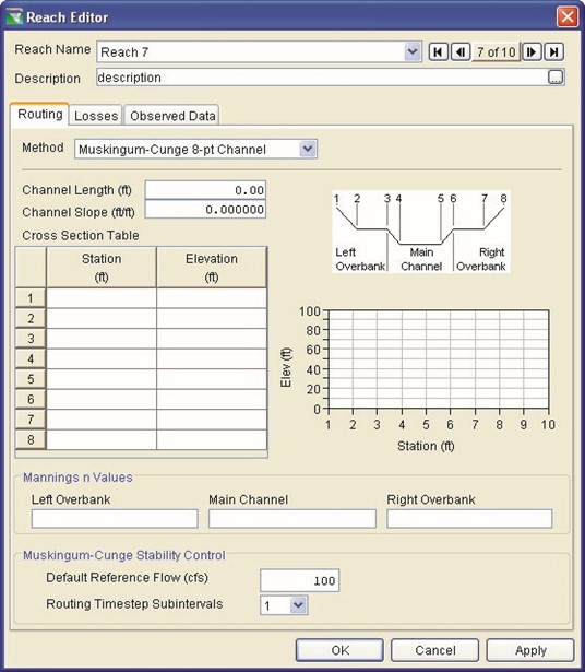
Figure 9.8 Reach Editor: Muskingum-Cunge 8-pt Channel

Routing Method

Channel Length: Enter the length of the routing reach.
Channel Slope: Enter the slope of the routing reach, ∆y/∆x.
Station: Enter the horizontal position of a point used to describe a stream cross section.
Elevation: Enter the vertical position of a point used to describe a stream cross section.
Manning's n Values: Enter the unitless loss coefficients for Left Overbank, Main Channel, and Right Overbank to be used in the normal depth calculations of the cross section.
Default Reference Flow: The flow value is used to compute the celerity (and thus the travel time) for the reach. If the travel time is less than the time-step size, the reach is divided into subreaches for the computation. Travel time (and thus the number of subreaches) is greater for low flow; therefore, the reference flow value should approximate the base flow for the reach.
Routing Timestep Subintervals: Select a value from 1 to
12.

To edit another reach without exiting the Reach Editor, click the Apply button and then select another reach from the Name list or use the navigator buttons.

9.2.1.4 Muskingum-Cunge Prismatic Channel Routing Method

The Muskingum-Cunge Prismatic Channel method (Figure 9.9) provides two more options for describing the cross section to be used by the Muskingum-Cunge hydrologic routing method. In this method, you can describe the cross section as either a trapezoid or a circle.

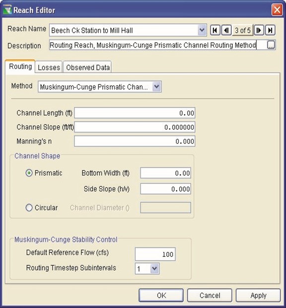
Figure 9.9 Reach Editor: Muskingum-Cunge Prismatic Channel

Routing Method

For the Muskingum-Cunge Prismatic Channel method, enter the appropriate parameters, described below:

Channel Length: Enter the length of the routing reach.
Channel Slope: Enter the slope of the routing reach, ∆y/∆x.
Manning's n: Enter the unitless loss coefficient to be used
in the normal depth calculations of the cross section.
Channel Shape: Select either Prismatic (trapezoid) or Circular (pipe).
- Prismatic: This shape is a basic trapezoid with the bottom of the trapezoid less than or equal to the width of the top. When you choose Prismatic as the Channel Shape, you also need to specify the Bottom Width and Side Slope.
  - Bottom Width: the width of the bottom of the trapezoidal section.
  - Side Slope: the slope of the sides of the trapezoid entered as ∆x/∆y.
- Circular: This shape is a simple circle used to represent a pipe or culvert. This method is valid for flow depth up to 0.77*diameter. For depths greater than this, the depth used by the method is held to 0.77*diameter and a warning message is generated. If you choose Circular as the Channel Shape, you also need to specify the Channel Diameter.
  - Channel Diameter: Define the size of the circle.
Muskingum-Cunge Stability Control: Enter the default reference flow and the routing timestep subintervals.
- Default Reference Flow: The flow value is used to compute the celerity (and thus the travel time) for the reach. If the travel time is less than the time step size, the reach is divided into subreaches for the computation. Travel time (and thus the number of subreaches) is greater for low flow; therefore, the reference flow value should approximate the base flow for the reach.
- Routing Timestep Subintervals: Select a value from 1 to 12.

To edit another reach without exiting the Reach Editor, click the Apply button and then select another reach from the Name list or use the navigator buttons.

9.2.1.5 Modified Puls Routing Method

The Modified Puls channel routing method (Figure 9.10) describes the reach as a set of cascading reservoirs, the number of which is specified by the number of subreaches. The outflow from the reach is defined as a function of the storage. An option is available within this method to account for seepage losses within the routing computation. To use this option, check the With Channel Losses box and enter the average Invert Elevation of the reach, the Percolation Rate to describe the seepage, and extend the outflow-storage table by adding associated elevation data.

If you use the Channel Losses option in this method, do not define seepage losses on the losses tab for this reach – you will be double accounting for the seepage losses.

Figure 9.10 Reach Editor: Modified Puls Routing Method

Storage: Enter monotonically increasing values of storage to describe the storage-outflow relationship needed for this routing method.
Outflow: Enter the outflow values associated with each
storage value in the storage-outflow relationship.
Elevation: Enter associated elevation values; ResSim uses these values as extensions to the storage-outflow relationship when you select the With Channel Losses option. This column is only available when this option is active.
Number of Subreaches: This parameter is similar to that used in the Muskingum routing method. Enter the reach travel time divided by the computation interval.
Invert Elevation: Enter the average minimum elevation of the channel in this reach.
Percolation Rate: Enter the flow rate identifying the loss of water to the soil/groundwater.
In the Select Plot area, you can choose whether the plot shows Storage vs. Outflow or Storage vs. Elevation. The plot will reflect the values you enter.

To edit another reach without exiting the Reach Editor, click the Apply button and then select another reach from the Name list or use the navigator buttons.

9.2.1.6 SSARR Routing Method

The SSARR routing method (Figure 9.11) describes the channel routing based on the computer program Streamflow Synthesis & Reservoir Regulation (SSARR), from the Corps' Northwestern Division (USACE, 1991).

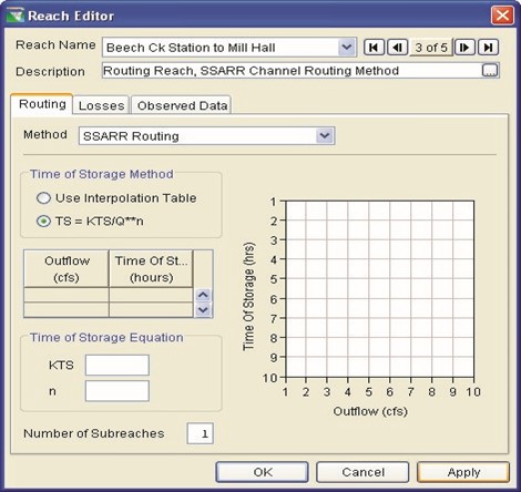
Figure 9.11 Reach Editor: SSARR Routing Method

The storage in the routing reach is defined by Time of Storage values (T_s), in units of hours. Therefore, the storage is defined like Muskingum K values (described in Section 9.2.1.2). Instead of using Modified Puls storage-outflow, this method uses T_s versus outflow.

An alternative method for defining T_s is by the following equation, which defines T_s as a power function of flow.

T_s= KTS_Qn

where:
T_s	=	Time of storage per increment in hours
KTS	=	Constant determined by trial and error or estimated from physical measurements of flow and corresponding routing times.
Q	=	Discharge in cubic meters (or feet) per hour
n	=	Coefficient usually between -1 and 1

As evident from the above equation, T_s is a nonlinear function of discharge except when n = 1. It is possible to use a negative value of n if time of storage increases as discharge increases. According to the SSARR User's Manual, a value of n = 0.2 is reasonable for most streams in the Columbia River Basin.

For the SSARR routing method, enter the appropriate parameters, described below:

Time of Storage Method: Select either the Use Interpolation Table or the TS = KTS/Qⁿ method.
Outflow and Time of Storage: If the Use Interpolation Table method is selected, enter the outflow and corresponding T_s values.
Time of Storage Equation: If the TS = KTS/Qⁿ method is selected, enter values for KTS and n.
Number of Subreaches: Number of steps applicable for the routing reach.

To edit another reach without exiting the Reach Editor, click the Apply button and then select another reach from the Name list or use the navigator buttons.

9.2.1.7 Working R&D Routing Method

The Working R&D routing method (Figure 9.12) uses a nonlinear storage-outflow relation, like the Modified Puls method. Also, it permits use of wedge storage, like the Muskingum method. For a linear storage-outflow relation, the Working R&D method produces results identical to the Muskingum method. For routing with no wedge storage (Muskingum X = 0), the Working R&D method produces results identical to the Modified Puls method (USACE, 1994).

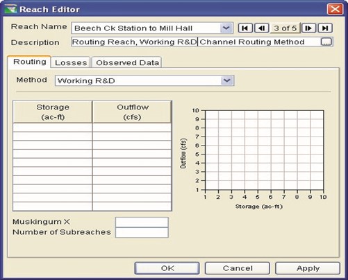
Figure 9.12 Reach Editor: Working R&D Routing Method

Storage: Enter monotonically increasing values of storage to describe the storage-outflow relationship needed for this routing method.
Outflow: Enter the outflow values associated with each storage value in the storage-outflow relationship.
Muskingum X: Enter the attenuation coefficient (from 0.0 to 0.5). A value of 0.0 indicates maximum attenuation of the hydrograph through the routing reach. A value of 0.5 indicates a "direct translation" of the hydrograph through the reach.
Number of Subreaches: Number of steps (subreaches) applicable for the routing reach. This parameter should be approximately equal to travel time divided by the computation interval.

To edit another reach without exiting the Reach Editor, click the Apply button and then select another reach from the Name list or use the navigator buttons.

9.2.1.8 Variable Lag & K

The Lag & K method is a hydrologic storage routing method for use between flow points that is based on a graphical routing technique. This method was incorporated into ResSim from the National Weather Service for use in specific watershed projects where Lag & K was the method used to calculate the original data. Lag & K is a flexible method of storage routing, where both Lag and K values can be either constant or variable. With constant Lag, all flows will be delayed with the same time in hours consistently. Variable Lag is determined from historical records, and it is a function of the inflow rate. Lag & K works by delaying the inflow hydrograph in time causing a lag in the graph. The K value is then used to attenuate the newly shifted curve.

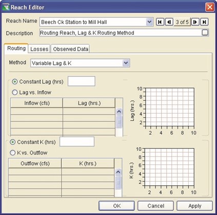
Figure 9.13 Reach Editor: Variable Lag & K Method

Constant Lag (hrs): enter the number of hours for the lag value
Lag vs. Inflow: enter your specific values for lag and inflow
Constant K (hrs): enter the number of hours for the K value
K vs. Outflow: enter your specific values for K and outflow

The continuity equation used to describe the K value is:

I – O = ds/dt

Where:

I = Inflow rate O = Outflow rate s = storage

t = time (∆t = routing interval)

9.2.2 Reach Editor: Losses Tab

The Losses tab of the Reach Editor (Figure 9.13) provides two options for computing losses in the routing reach: Constant Seepage or Seepage as a function of Flow. The default is no losses in the reach.

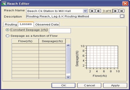
Figure 9.14 Reach Editor: Losses Tab

Constant Seepage: Enter the flow (in cms or cfs) lost to the reach through the soil, non-varying throughout the simulation.
Seepage as a function of Flow: With this option, you can define the loss as a function of the routed flow of the reach. Reach losses are computed after the flow is routed through the reach; therefore, the final outflow from the reach is the routed flow minus the loss.
Flow: Enter a monotonically increasing set of flow values to define the relationship of seepage with respect to flow.
Seepage: Enter the associated seepage values for each flow value in the table, expressed in flow units.

The mini-plot will reflect the values you enter and can be viewed in full size when you double-click on it.

To edit another reach without exiting the Reach Editor, click the Apply button and then select another reach from the Name list or use the navigator buttons.

9.2.3 Reach Editor: Observed Data Tab

Use the Observed Data tab (Figure 9.14) to indicate that observed data is available for comparison purposes. If the Observed box in the table is checked (as shown in Figure 9.14), then there will be a corresponding entry in the Observed Time-Series mapping table when you create an Alternative (Chapter 13).

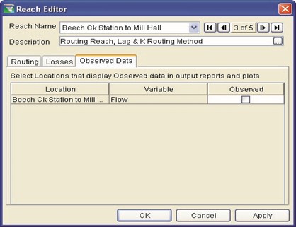
Figure 9.15 Reach Editor: Observed Data Tab

To edit another reach without exiting the Reach Editor, click the Apply button and then select another reach from the Name list or use the navigator buttons.

9.3 Editing Diversion Properties

To edit diversion data, select the Diversion Tool and right-click on a diversion. From the shortcut menu, select Edit Diversion Properties. The Diversion Editor will open (Figure 9.15).

Figure 9.16 Diversion Editor

The Name field at the top of the Editor contains a list of all of the diversions in your reservoir network, with the name of the current diversion displayed. You can access all of the diversions both from this list and by using the VCR-style buttons to navigate through the available diversions.

If the Computed during UnReg box is checked, then the diversion will operate during the unregulated flow calculation. If the box is left unchecked, then the unregulated flow will reflect flow conditions without the diversion.

The Diversion Editor has four tabs that allow you to edit diversion information (Diversion tab), Losses, Routing, and Observed Data, as described in the following sections.

Note that the Losses and Routing tabs are available only for diversions that connect to downstream nodes.

9.3.1 Diversion Editor: Diversion Tab

The Diversion Editor's Diversion tab allows you to choose from seven methods: Constant, Monthly Varying, Seasonal,

Function of Flow, Function of

Pool Elevation, Time Series, and Flexible Diversion Rule; each with its own parameters. The default method is Constant.

Select the diversion method from the Method list. The appropriate editing fields will appear according to the method you have selected.

9.3.1.1 Constant Diversion Method

For the Constant method (Figure 9.16), you will need to enter a diversion flow value (in the appropriate units of your watershed). This constant value will apply to each period of your simulation.

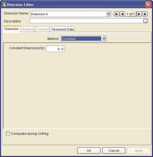
Figure 9.17 Diversion Editor: Constant Diversion Method

To edit another diversion without exiting the Diversion Editor, click the Apply button and then select another diversion from the Diversion Name list or use the navigator buttons.

9.3.1.2 Monthly Varying Diversion Method

For the Monthly Varying diversion method (Figure 9.17), you will need to enter the diversion flow value (in the appropriate units of your watershed) corresponding to each month of a year. These monthly values will apply to each year in your simulation.

Figure 9.18 Diversion Editor: Monthly Varying

Diversion Method

Diversion: Enter a flow value (in cms or cfs) for each month.

To edit another diversion without exiting the Diversion Editor, click the Apply button and then select another diversion from the Diversion Name list or use the navigator buttons.

9.3.1.3 Seasonal Diversion Method

For the Seasonal method (Figure 9.18), you will need to enter a Date along with a corresponding Diversion flow value (in the appropriate units of your watershed). The seasonal diversion is applicable for each year of your simulation.

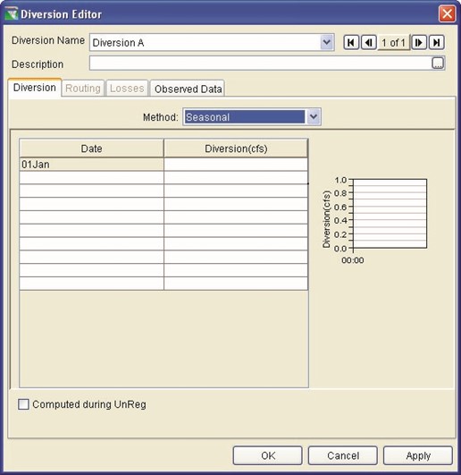
Figure 9.19 Diversion Editor: Seasonal Diversion Method

Date: Enter the Day and Month in the format ddMMM
(e.g., 01Jan).
Diversion: Enter a Flow value in cms or cfs.

To edit another diversion without exiting the Diversion Editor, click the Apply button and then select another diversion from the Diversion Name list or use the navigator buttons.

9.3.1.4 Function of Flow Diversion Method

For the Function of Flow diversion method (Figure 9.19), you will need to enter a relationship between a junction's net flow and the resulting diverted flow (in the appropriate units of your watershed). The Flow Location junction can be selected from the list and need not be the same location as where the diversion occurs. This allows for a diversion to limit or augment flow based on any junction's flow. For a given net Flow value entering the diversion element, the Diversion flow will be removed from the junction. This relationship applies to your entire Simulation period.

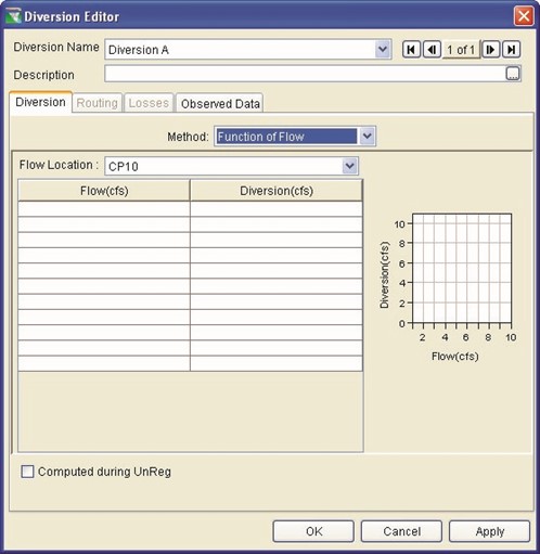
Figure 9.20 Diversion Editor: Function of Flow

Diversion Method

Flow: Enter the net flow (in cms or cfs) entering the junction.
Diversion: Enter the flow (in cms or cfs) that is diverted from the junction.

To edit another diversion without exiting the Diversion Editor, click the Apply button and then select another diversion from the Diversion Name list or use the navigator buttons.

9.3.1.5 Function of Pool Elevation Diversion Method

For the Function of Pool Elevation diversion method (Figure 9.20), you will need to enter a relationship between reservoir elevation and diversion flow (in the appropriate units of your watershed). Also, you will need to select the appropriate reservoir from the Reservoir list. When a given Elevation at the selected reservoir occurs, then the corresponding Diversion flow will be diverted from the junction. Linear interpolation will be made between the elevations (and corresponding diversions) that you enter.

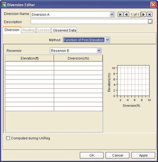
Figure 9.21 Diversion Editor: Function of Pool Elevation

Diversion Method

Elevation: Enter the reservoir elevation (in meters or feet) on which the diversion is based.
Diversion: Enter the flow (in cms or cfs) that is diverted from the diversion element.

To edit another diversion without exiting the Diversion Editor, click the Apply button and then select another diversion from the Diversion Name list or use the navigator buttons.

9.3.1.6 Time-Series Diversion Method

For the Time-Series diversion method (Figure 9.21), you only need to select Time Series from the Method list. An entry for this diversion will appear in the Time-Series mapping table when you create an Alternative (Chapter 13). The time series of diversion flow values must be in the appropriate units (cms or cfs) of your watershed.

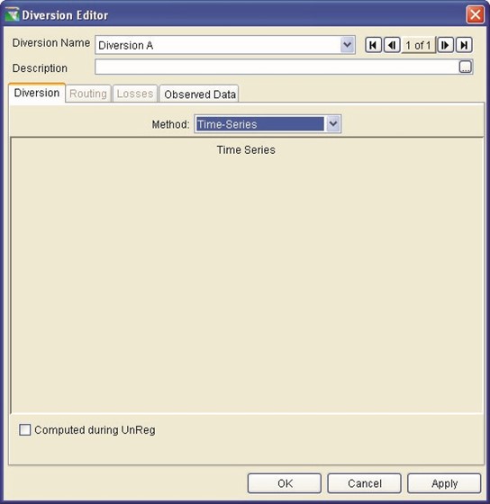
Figure 9.22 Diversion Editor: Time-Series Diversion Method

To edit another diversion without exiting the Diversion Editor, click the Apply button and then select another diversion from the Diversion Name list or use the navigator buttons.

9.3.1.7 Flexible Diversion Rule Method

The Flexible Diversion Rule diversion method (Figure 9.23) brings more utility to the use of a diversion, puts more power in the hands of the modeler, and brings the capabilities of ResSim diversion modeling to the next level. It essentially combines all other diversion methods to allow the diversion to behave similar to a reservoir release function rule (Chapter 11, Section 11.5.3) and allows the user to have scripting abilities.

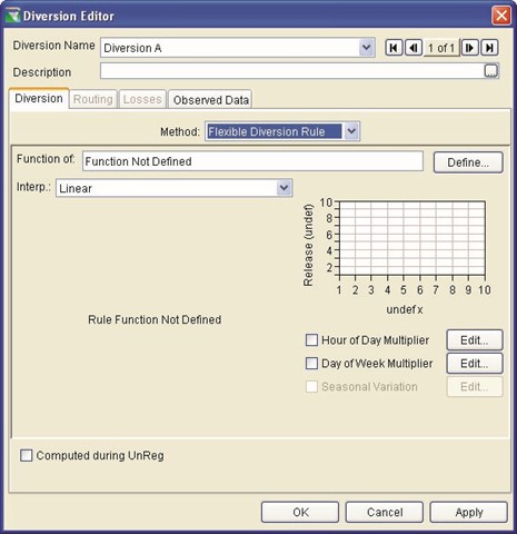
Figure 9.23 Diversion Editor: Flexible Diversion Rule Method

1. Click the

"Function of:" Define… button. The Independent Variable Definition editor will open (Figure 9.24) where you can select from the following "Release is a function of" options: Date, Date and Time,

Model Variable, External Variable, and State Variable.

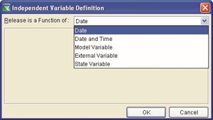
Figure 9.24 Diversion Editor:

Flexible Diversion Rule –

Select Independent Variable

2. If the function type is Date, the editor (Figure 9.25) will appear for you to enter the appropriate dates and diversion flow (in the Release column). You can enter a single value for 01 Jan to describe a constant diversion amount throughout the year or enter multiple dates to define a seasonally varying diversion.

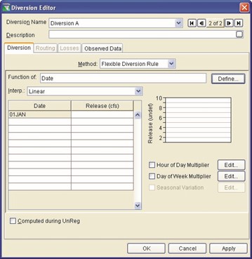
Figure 9.25 Diversion Editor:

Flexible Diversion--Function of Date

This function is similar to the Constant (Section 9.3.1.1) and Seasonal (Section 9.3.1.3) diversion methods, but includes additional options for Hour of Day and Day of Week Multipliers.

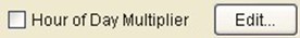The Hour of Day Multiplier allows you to specify a factor (based on the time of day) that will be applied to the diversion. To do this, click on the Hour of Day Multiplier Edit button. The Hour of Day Multiplier editor will appear where you will see that the default value for all hours of the day is 1.0 (Figure 9.26). If you have a diversion that diverts only during a portion of the day, you can set the multiplier for those hours to 1.0 and set all other hours to 0.0. For example, to specify that a diverted flow would only occur from 8:00 a.m. to 5:00 p.m., change the value of 1.0 to 0.0 for hours 0000-0800 and 1700-2400. If you want to increase the diversion flow by 50% between 8:00 a.m. and 5:00 p.m., then enter a factor of 1.5 for hours 0800-1700 (Figure 9.27).

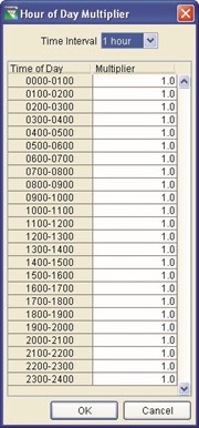
Figure 9.26 Hour of Day Multiplier with Default Values of 1.0 Specified for Entire Day

Figure 9.27 Hour of Day

Multiplier with Values of 1.5

Click OK to close the Hour of Day Multiplier editor.

In the diversion editor,

the check box in front of the Hour of Day Multiplier will display a check mark only when the default set of multipliers is modified.

The Day of Week Multiplier allows you to specify a factor (based on the day of the week) that will be applied to the diversion flow. To do this, click on the Day of Week Multiplier Edit button. The Day of Week Multiplier editor will appear (Figure 9.28) where you will see that the default value is 1.0 for all days of the week (Sunday through Saturday). If you have a diversion that diverts only during Monday through Friday, you can set the multiplier for Saturday and Sunday to 0.0 and leave all other days set to 1.0 (Figure 9.29). If you want to increase the diversion flow relative to other flows in the pattern by 50% on Wednesday, then enter a factor of 1.5 for Wednesday.

Specified for Portion of Day

Figure 9.28 Day of Week

Multiplier with Default

Factors of 1.0 Specified for

Each Day of the Week

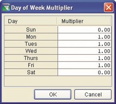
Figure 9.29 Day of Week

Multiplier with Factors of 0.0

Specified for Saturday and

Sunday

Click OK to close the Day of Week Multiplier editor.

In the diversion editor,

the check box in front of

Day of Week Multiplier will display a check mark only when the default set of multipliers is modified.

If the function type is Date and Time, the editor (Figure 9.30) will appear for you to enter the appropriate dates and times along with the diversion flow (in the Release column).

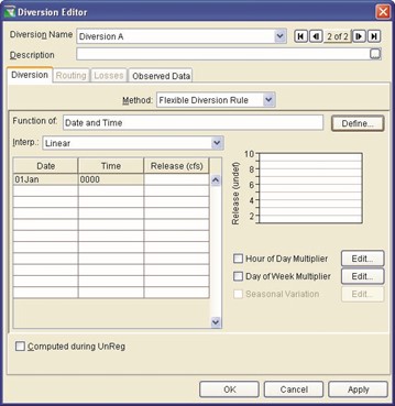
Figure 9.30 Diversion Editor:

Flexible Diversion--Function of Date & Time

If the function type is Model Variable, select the independent variable using the scrollable list and/or using the Filter chooser (Figure 9.31).

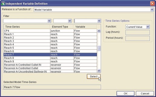
Figure 9.31 Diversion Editor: Flexible Diversion-- Function of Model Variable

If the function type is External Variable, identify the independent variable in the Variable Name field (Figure 9.32). This name will appear on the time-series tab of the Alternative

Editor (Chapter 13, Section 13.8).

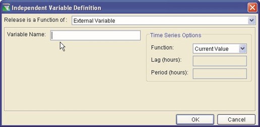
Figure 9.32 Diversion Editor: Flexible Diversion--

Function of External Variable

If the function type is State Variable, select the State Variable from the list (Figure 9.33). The state variable must be defined prior to creating a flexible diversion function that uses it (see documentation of State Variables in Section 11.13.1).

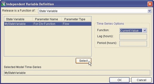
Figure 9.33 Diversion Editor: Flexible Diversion--

Function of State Variable

If the function type is Model Variable, External Variable, or State Variable, to define the independent variable with respect to each time step, you should choose the appropriate function from Time Series Options. From the Function list (Figure 9.34), you can select: Current Value, Previous Value,
Lagged Value, Period Average, Period Maximum, or Period
Minimum. The Lag (in hours) can be specified (for all but Current and Previous value) along with the appropriate Period (in hours).

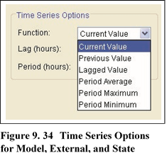
Variable Independent Variables

To edit another diversion without exiting the Diversion Editor,

click the Apply button and then select another diversion from the

Diversion Name list or use the navigator buttons.

9.3.2 Diversion Editor: Routing Tab

For diversions connected to downstream junctions, the Diversion Editor's Routing tab allows you to choose from eight routing methods: Coefficient, Muskingum, Muskingum-Cunge 8-pt Channel, Muskingum-Cunge Prismatic Channel, Modified Puls, SSARR, Working R&D Routing, and Variable Lag & K; each with its own set of parameters. If there is no lag or translation of the hydrograph through the diversion reach, you can select Null Routing (which is the default routing method).

The Routing tab of the Diversion Editor is identical to the Routing tab of the Reach Editor. For details about using the Routing tab, refer to Section 9.2.1.

9.3.3 Diversion Editor: Losses Tab

Available for diversions connected to a downstream junction, the Losses tab of the Diversion Editor (Figure 9.35) provides three options for computing losses in the diversion's routing reach: Return Ratio, Constant Seepage, or Seepage as a function of Flow.

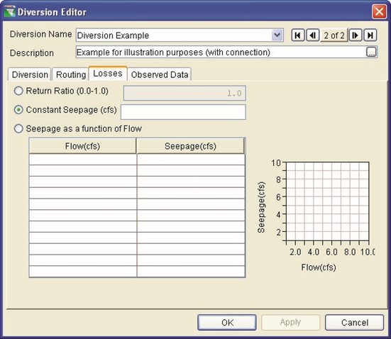
Figure 9.35 Diversion Editor: Losses Tab

Return Ratio: Enter a value between 0.0 and 1.0 (the default is 1.0) to indicate how much diversion continues through the diversion to the downstream junction.
Constant Seepage: Enter a seepage value (in cms or cfs) to indicate how much diversion flow will "seep into" the ground and therefore be lost from the system.
Seepage as a function of Flow: Enter a Flow vs. Seepage relationship (in cms or cfs) to indicate how much of the diversion flow is lost from the diversion to the ground.

The mini-plot will reflect the values you enter and can be viewed in full size when you double-click on it.

To edit another diversion without exiting the Diversion Editor, click the Apply button and then select another diversion from the Diversion Name list or use the navigator buttons.

9.3.4 Diversion Editor: Observed Data Tab

Use the Observed Data tab (Figure 9.36) to indicate that observed data is available for comparison purposes. If the Observed box in the table is checked, then there will be a corresponding entry in the Observed Time-Series mapping table when you create an Alternative (Chapter 13).

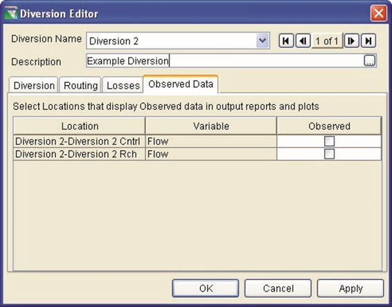
Figure 9.36 Diversion Editor: Observed Data Tab

To edit another diversion without exiting the Diversion Editor, click

the Apply button and then select another diversion from the

Diversion Name list or use the navigator buttons.

– Defining Physical Components of Reservoirs

Chapter 10

Defining Physical Components of Reservoirs

Section Page

10 DEFINING PHYSICAL COMPONENTS OF RESERVOIRS............................... 10-1

10.1 ACCESSING THE RESERVOIR EDITOR ........................................................ 10-2

10.2 USING THE RESERVOIR EDITOR TO DEFINE PHYSICAL COMPONENTS .......... 10-2

10.3 SPECIFYING PHYSICAL COMPONENTS OF A RESERVOIR ............................. 10-3 10.4 SPECIFYING RESERVOIR POOL LOSSES .................................................... 10-4 10.5 DEFINING PHYSICAL FEATURES OF A DAM ................................................. 10-4 10.6 ADDING LEAKAGE TO A DAM ..................................................................... 10-5 10.7 ADDING OUTLET GROUPS ........................................................................ 10-6 10.8 DEFINING CONTROLLED OUTLETS ............................................................. 10-7

10.8.1 ADDING CONTROLLED OUTLETS ................................................. 10-7 10.8.2 ADDING POWER PLANTS ............................................................ 10-8 10.8.3 ADDING PUMPS ......................................................................... 10-9

10.9 ADDING UNCONTROLLED OUTLETS ......................................................... 10-10 10.10 ADDING TAILWATER ELEVATION .............................................................. 10-11

10.11 DEFINING PHYSICAL COMPONENTS OF A DIVERTED OUTLET ..................... 10-12

10.12 RENAMING, DELETING, AND REMOVING RESERVOIR COMPONENTS ........... 10-13

10.12.1 RENAMING RESERVOIR COMPONENTS ...................................... 10-13 10.12.2 DELETING RESERVOIR COMPONENTS ....................................... 10-14 10.12.3 REMOVING RESERVOIR PARAMETERS....................................... 10-15

10.13 EDITING RESERVOIR PHYSICAL DATA ...................................................... 10-15 10.14 EDITING POOL PHYSICAL DATA ............................................................... 10-16

10.14.1 EDITING POOL EVAPORATION DATA .......................................... 10-17 10.14.2 EDITING POOL SEEPAGE .......................................................... 10-18

10.15 EDITING DAM LEAKAGE .......................................................................... 10-19 10.16 EDITING CONTROLLED OUTLET PHYSICAL DATA ...................................... 10-20

10-i

10.17 EDITING POWER PLANT PHYSICAL DATA ................................................. 10-22

10.17.1 EDITING OUTLET CAPACITY DATA FOR A POWER PLANT ............ 10-22

10.17.5 EDITING HYDRAULIC LOSSES DATA FOR A POWER PLANT .......... 10-32

10.18 EDITING PUMP PHYSICAL DATA .............................................................. 10-34

10.18.1 PUMP CAPACITY AS CONSTANT ................................................ 10-34

10.18.2 PUMP CAPACITY AS FUNCTION OF OPERATING HEAD ................ 10-35

10.19 EDITING UNCONTROLLED OUTLET PHYSICAL DATA .................................. 10-36 10.20 EDITING TAILWATER ELEVATION PHYSICAL DATA ..................................... 10-37 10.21 VIEWING COMPOSITE RELEASE CAPACITY TABLES .................................. 10-39

10.21.1 RESERVOIR COMPOSITE RELEASE CAPACITY TABLE ................. 10-39

10.21.2 DAM COMPOSITE RELEASE CAPACITY TABLE ............................ 10-40

10.21.3 DIVERTED OUTLET COMPOSITE RELEASE CAPACITY TABLE ....... 10-40 10.21.4 OUTLET GROUP COMPOSITE RELEASE CAPACITY TABLE ........... 10-40

10.22 RESERVOIR EDITOR: PULSE FLOW OPTIONS ........................................... 10-41 10.23 RESERVOIR EDITOR: OBSERVED DATA TAB ............................................ 10-42

List of Figures

Figure Page Number

FIGURE 10.1 RESERVOIR EDITOR: PHYSICAL TAB ....................................................... 10-2

FIGURE 10.2 RESERVOIR EDITOR, PHYSICAL TAB: DEFAULT RESERVOIR

COMPONENT TREE ........................................................................... 10-3

FIGURE 10.3 RESERVOIR EDITOR, PHYSICAL TAB: DEFAULT RESERVOIR

COMPONENT TREE WITH DIVERTED OUTLET ...................................... 10-3

FIGURE 10.4	RESERVOIR EDITOR, PHYSICAL TAB: WITH POOL LOSSES ....................... 10-4
FIGURE 10.5	RESERVOIR EDITOR: POOL MENU ......................................................... 10-4
FIGURE 10.6	RESERVOIR TREE: POOL SHORTCUT MENU ........................................... 10-4
FIGURE 10.7	RESERVOIR TREE: DAM ........................................................................ 10-4
FIGURE 10.8	RESERVOIR EDITOR, PHYSICAL TAB: DAM MENU ................................... 10-5
FIGURE 10.9	RESERVOIR TREE: DAM SHORTCUT MENU ............................................. 10-5

FIGURE 10.10 RESERVOIR TREE: OUTLET GROUPS ..................................................... 10-6 FIGURE 10.11 DIVERTED OUTLET SHORTCUT MENU: ADD OUTLET GROUP ................... 10-6

FIGURE 10.12 RESERVOIR TREE: CONTROLLED OUTLETS, POWER PLANTS AND

PUMPS...........................................................................................1 0-7

FIGURE 10.13 DAM SHORTCUT MENU: ADD CONTROLLED OUTLET ............................... 10-7 FIGURE 10.14 DAM SHORTCUT MENU: ADD POWER PLANT .......................................... 10-8 10-ii

Defining Physical Components of Reservoirs

FIGURE 10.15 DAM SHORTCUT MENU: ADD PUMP ....................................................... 10-9 FIGURE 10.16 RESERVOIR TREE: UNCONTROLLED OUTLETS ...................................... 10-10 FIGURE 10.17 DAM SHORTCUT MENU: ADD UNCONTROLLED OUTLET ......................... 10-10 FIGURE 10.18 RESERVOIR TREE: TAILWATER ELEVATION .......................................... 10-11 FIGURE 10.19 DAM SHORTCUT MENU: ADD TAILWATER ELEVATION ........................... 10-11

FIGURE 10.20 RESERVOIR TREE: DIVERTED OUTLET ................................................. 10-12 FIGURE 10.21 RESERVOIR EDITOR: OUTLET MENU FOR DIVERTED OUTLET ................ 10-12 FIGURE 10.22 RESERVOIR COMPONENT SHORTCUT MENU: RENAME COMPONENT ...... 10-13

FIGURE 10.23 RENAME RESERVOIR COMPONENT....................................................... 10-13

FIGURE 10.24 RESERVOIR COMPONENT SHORTCUT MENU: DELETE COMPONENT ....... 10-14 FIGURE 10.25 CONFIRM DELETION OF RESERVOIR COMPONENT ................................. 10-14 FIGURE 10.26 RESERVOIR PARAMETER SHORTCUT MENU: REMOVE PARAMETER ....... 10-15 FIGURE 10.27 CONFIRM REMOVAL OF RESERVOIR PARAMETER .................................. 10-15 FIGURE 10.28 RESERVOIR EDITOR: PHYSICAL DATA -- POOL ..................................... 10-16 FIGURE 10.29 RESERVOIR EDITOR: PHYSICAL DATA -- POOL EVAPORATION ............... 10-17 FIGURE 10.30 RESERVOIR EDITOR: PHYSICAL DATA -- POOL SEEPAGE ...................... 10-18 FIGURE 10.31 RESERVOIR EDITOR: PHYSICAL DATA -- DAM LEAKAGE ........................ 10-19 FIGURE 10.32 CONTROLLED OUTLET (NO GATE SETTINGS) ........................................ 10-20 FIGURE 10.33 GATE SETTINGS .................................................................................. 10-21 FIGURE 10.34 CONTROLLED OUTLET (WITH GATE SETTINGS) ..................................... 10-21 FIGURE 10.35 POWER PLANT PHYSICAL DATA EDITOR: OUTLET TAB .......................... 10-22 FIGURE 10.36 POWER PLANT PHYSICAL DATA EDITOR: CAPACITY TAB ....................... 10-23 FIGURE 10.37 POWER PLANT CAPACITY TAB: VARIABLE CAPACITY OPTIONS .............. 10-23 New

FIGURE 10.38 POWER PLANT CAPACITY TAB: VARIABLE CAPACITY --

FUNCTION OF RESERVOIR ELEVATION ........................................... 10-24 New

FIGURE 10.39 POWER PLANT CAPACITY TAB: VARIABLE CAPACITY --

FUNCTION OF RESERVOIR STORAGE ............................................. 10-24 New

FIGURE 10.40 POWER PLANT CAPACITY TAB: VARIABLE CAPACITY --

FUNCTION OF RELEASE ................................................................ 10-25 ^New

FIGURE 10.41 POWER PLANT CAPACITY TAB: VARIABLE CAPACITY --

FUNCTION OF OPERATING HEAD ................................................... 10-25^New

FIGURE 10.42 POWER PLANT PHYSICAL DATA EDITOR: EFFICIENCY TAB --

CONSTANT EFFICIENCY METHOD .................................................. 10-26

FIGURE 10.43 POWER PLANT PHYSICAL DATA EDITOR: EFFICIENCY TAB --

FUNCTION OF RESERVOIR ELEVATION ........................................... 10-27

FIGURE 10.44 POWER PLANT PHYSICAL DATA EDITOR: EFFICIENCY TAB --

FUNCTION OF RELEASE ................................................................ 10-28

FIGURE 10.45 POWER PLANT PHYSICAL DATA EDITOR: EFFICIENCY TAB --

FUNCTION OF OPERATING HEAD ................................................... 10-29

FIGURE 10.46 POWER PLANT PHYSICAL DATA EDITOR: STATION USE TAB --

CONSTANT METHOD .................................................................... 10-30

FIGURE 10.47 POWER PLANT PHYSICAL DATA EDITOR: STATION USE TAB --

FUNCTION OF RELEASE METHOD .................................................. 10-31

10-iii

FIGURE 10.48 POWER PLANT PHYSICAL DATA EDITOR: HYDRAULIC LOSSES TAB --

CONSTANT METHOD .................................................................... 10-32

FIGURE 10.49 POWER PLANT PHYSICAL DATA EDITOR: HYDRAULIC LOSSES TAB --

FUNCTION OF RELEASE METHOD .................................................. 10-33

FIGURE 10.50 PUMP PHYSICAL DATA EDITOR: PUMP CAPACITY -- CONSTANT ............. 10-34 FIGURE 10.51 PUMP PHYSICAL DATA EDITOR: PUMP CAPACITY --

FUNCTION OF OPERATING HEAD ................................................... 10-35

10-iv

Defining Physical Components of Reservoirs

CHAPTER 10

Defining Physical Components of Reservoirs

The data that defines an individual reservoir element within the reservoir network consists of two conceptual types: Physical and Operational. This chapter describes the physical components of a reservoir that include the Pool, the Dam (and its Outlets), and any Diverted Outlets (commonly called diversions from the pool). ResSim represents these components using a "tree structure". As you add optional physical components to the reservoir, they will appear in the reservoir tree. This reservoir tree is more than just an illustration. It is the mechanism you will use to access the editors for the separate reservoir components. As you select a component in the reservoir tree, the edit panel to the right of the reservoir tree will display the editor you need to define the properties of that component.

An elevation-storage-area relationship describes the properties of the pool, while a crest elevation and length describes the dam, represented internally in the ResSim program as an uncontrolled spillway. You will need to add one or more outlets to the dam to enable water to pass through it into the downstream system. You can also add a power plant to describe the hydropower generating capacity. Within the Reservoir Editor, Diverted Outlets (or reservoir diversions) are separate outlet groups. As with the dam, you will need to add one or more outlets to a diverted outlet group to enable the reservoir to allocate flow through the diversion.

The order in which you add physical components and edit their properties is flexible. You can add all the physical components to the reservoir then go back and define each component's properties, or you can define the properties of each component as you add it, before going on to add and edit the next component. Choose the style that works best for you. However, you should finish defining the physical representation of your reservoir before going on to define its operational data (Chapter 11), as the definition of the operational zones depends on the physical definition of the pool, and the rules depend on the description of the outlet works.

10.1 Accessing the Reservoir Editor

In the Reservoir Network Module, you can access the Reservoir Editor from either the Edit menu in the menu bar or from the right-click shortcut menu of a reservoir in the map display.

From the Edit menu, select Reservoirs....
From the map display, right-click on a reservoir with the
Reservoir Tool , then select Edit Reservoir Properties.

10.2 Using the Reservoir Editor to Define Physical Components

The Physical tab of the Reservoir Editor allows you to define the physical properties of reservoirs in your reservoir network. Figure 10.1 shows the Reservoir Editor with the Physical tab selected.

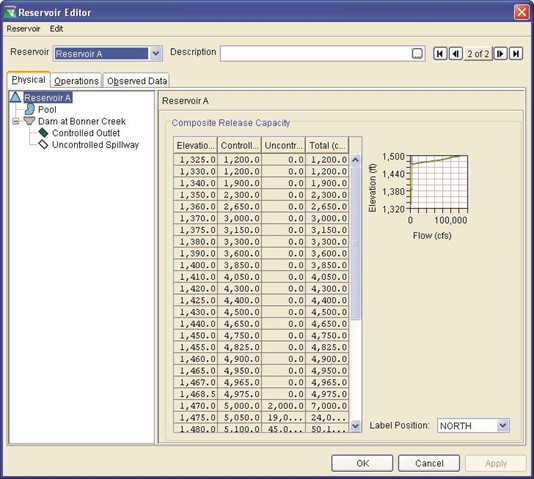
Figure 10.1 Reservoir Editor: Physical Tab

On the Physical tab, a reservoir tree appears in the left panel of the window. By default, the reservoir tree displays the reservoir and its primary components: the Pool and the Dam. Additionally, if you add a diversion to remove water from this reservoir's pool in the reservoir network, a Diverted Outlet appears in the reservoir tree. As you add components to the reservoir, such as outlets and losses, the reservoir tree will expand to show these components.

The area to the right of the reservoir tree is the Edit Panel. The content of this panel changes according to the component you select in the reservoir tree. Figure 10.1 shows the Composite Release Capacity summary for the reservoir because the reservoir is the selected component in the reservoir tree.

The menu bar of the Reservoir Editor changes according to the component you select in the reservoir tree. For example, when you select the Dam in the reservoir tree, a Dam menu becomes available in the menu bar.

When the reservoir is selected in the tree, you may re-position the name label in your map display by choosing from the options in the Label Position field (see the lower right portion of the editor in Figure 10.1).

The Reservoir field at the top of the Editor contains a list of all of the reservoirs in your network, with the name of the current reservoir displayed. You can access all of the reservoirs both from this list and by using the VCR-style buttons to navigate through the available reservoirs. Below the Reservoir name list is the Description of the current reservoir; this field is editable.

The following sections describe how to use the Physical tab of the Reservoir Editor to define the physical components of the reservoir that appear in the reservoir tree.

10.3 Specifying Physical Components of a Reservoir

On the Physical tab of the Reservoir Editor, a reservoir tree appears in the left panel of the window. By default,

the primary components for all

reservoirs are a Pool and a Dam, as

Figure 10.2 illustrates.

A Pool reflects characteristics of

Figure 10.2 Reservoir Editor,

Physical Tab: Default

Reservoir Component Tree

reservoir storage, while a Dam reflects the reservoir dam and its outlets.

Additionally, if the individual reservoir has a diverted outlet, a Diverted Outlet will appear as a primary component of the reservoir, as illustrated in Figure 10.3.

The Reservoir and primary components

that appear in the default reservoir tree are features of the reservoir network that you have setup previously using the map (mouse) tools. The following

Figure 10.3 Reservoir

Editor, Physical Tab: Default Reservoir Component Tree with Diverted Outlet

sections explain how to add details to the primary components of a reservoir and how to define secondary components such as outlets and losses.

10.4 Specifying Reservoir Pool Losses

You can specify both Pool Evaporation and Pool Seepage, as shown in Figure 10.4.

On the Physical tab, you may use either the Pool menu in the Reservoir Editor's menu bar (Figure 10.5) or the right-click shortcut menu (Figure 10.6) to specify Losses for a reservoir pool.

To add Pool Evaporation and/or Pool Seepage:

Select Pool in the reservoir tree.

Figure 10.4 Reservoir

Either click on Pool in the

Editor, Physical Tab: with

menu bar or right-click on Pool

Pool Losses

in the reservoir tree to access the shortcut menu.

Select Add Pool Evaporation or Add Pool Seepage.

Figure 10.5 Reservoir Editor: Figure 10.6 Reservoir Tree:

Pool Menu Pool Shortcut Menu

You can also remove Pool Seepage and Pool Evaporation, as described in Section 10.12.3.

10.5 Defining Physical Features of a Dam

As Figure 10.7 shows, you can add the following physical features to a Dam:

Leakage (Section 10.6),

Tailwater Elevation (Section 10.10),

Controlled Outlets (Section 10.8.1),

Uncontrolled Outlets (Section 10.9),

Outlet Groups (Section 10.7), Power Plants (Section 10.8.2), and Pumps (Section 10.8.3).

You can also rename Dams in the reservoir tree, as described in Section 10.12.1.

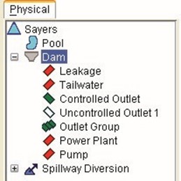
Figure 10.7 Reservoir Tree:

Dam

On the Physical tab, you may use either the Dam menu in the Reservoir Editor's menu bar (Figure 10.8) or the right-click shortcut menu (Figure 10.9) to specify features of a dam.

10.6 Adding Leakage to a Dam

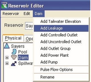To add Leakage to a dam:

Select the dam by clicking on it in the reservoir tree.

Select Add Leakage from either the Dam menu in the Reservoir Editor's menu bar (Figure 10.8) or the right-click shortcut
menu of the Dam

(Figure 10.9).

Figure 10.8 Reservoir Editor,

Physical Tab: Dam Menu

Leakage will now appear

as a "branch" of the

reservoir tree, beneath the dam.

You can also remove Leakage from a dam (Section 10.12.3).

Figure 10.9 Reservoir Tree:

Dam Shortcut Menu

10.7 Adding Outlet Groups

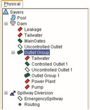You can add Outlet Groups as components of Dams, Diverted Outlets, and other Outlet Groups, as shown in Figure 10.10.

An Outlet Group allows you to define subsets of a reservoir component. An Outlet Group can include Tailwater Elevation

(Section 10.10), Controlled

Outlets (Section 10.8),

Uncontrolled Outlets (Section 10.9), and other Outlet Groups as components.

On the Physical tab, you may use either the component-specific menus in the Reservoir Editor's menu bar or the right-click shortcut

menus (Figure 10.11) to add an Outlet Group as a component of a Dam, Diverted Outlet, or other Outlet Group.

To add an Outlet Group:

Select the Dam, Diverted Outlet, or Outlet Group to which you want to add the new Outlet Group.
Choose Add Outlet Group from the shortcut menu (Figure 10.11) or from the component's menu in the Reservoir Editor's menu bar.

The new Outlet Group will appear in the reservoir

tree as a branch beneath the component you selected.

You can also rename and delete

Outlet Groups in the reservoir Figure 10.10 Reservoir Tree:

Outlet Groups

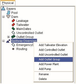
Figure 10.11 Diverted Outlet

Shortcut Menu:

Add Outlet Group

tree, as described in Section 10.12.

10.8 Defining Controlled Outlets

You can add Controlled Outlets,

Power Plants, and Pumps to Dams, Diverted Outlets, and Outlet Groups, as shown in Figure 10.12.

Additionally, you can add Tailwater Elevation (Section 10.10) as a component of Controlled Outlets, Power Plants, and Pumps.

You can also rename and delete

Controlled Outlets, Power Plants, and Pumps in the reservoir tree Figure 10.12 Reservoir Tree:

(Section 10.12). ^Controlled

Outlets, Power

Plants and

Pumps

10.8.1 Adding Controlled Outlets

On the Physical tab, you may use either the component-specific menus in the Reservoir Editor's menu bar or the right-click shortcut menus (Figure 10.13) to add a Controlled Outlet as a component of a Dam, Diverted Outlet, or Outlet Group.

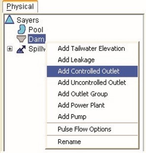To add a Controlled Outlet:

Select the Dam or Outlet Group to which you want to add the new
Controlled Outlet.
Choose Add Controlled Outlet from the shortcut menu (Figure 10.13) or from the
component's menu

in the Reservoir

Figure 10.13 Dam Shortcut Menu: Editor's menu bar.

Add Controlled Outlet

The new Controlled Outlet will appear in the

reservoir tree as a branch beneath the dam or outlet group you selected.

You can rename and delete Controlled Outlets (as described in Section 10.12).

10.8.2 Adding Power Plants

Power Plants are added in the same manner as the controlled outlets (as described in Section 10.8.1). Therefore, on the Physical tab, you may use either the component-specific menus in the Reservoir Editor's menu bar or the right-click shortcut menus (Figure 10.14) to add a Power Plant as a component of a Dam, Diverted Outlet, or Outlet Group.

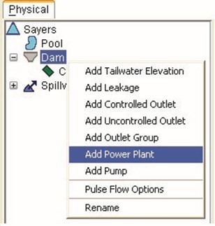To add a Power Plant:

Select the Dam or Outlet Group to which you want to add the Power Plant.
Select Add Power Plant from the shortcut menu (Figure 10.14) or from the component's menu in the Reservoir Editor's menu bar.

Figure 10.14 Dam Shortcut Menu:

Add Power Plant

The Power Plant will now appear as a branch of the reservoir tree, beneath the component that it was added to.

You can rename and delete Power Plants (as described in Section 10.12).

To properly calculate energy production, a power plant requires a tailwater definition to be with or above the power plant in the outlet tree. See Section 10.10 for a description of adding Tailwater Elevation.

10.8.3 Adding Pumps

Pumps are added in the same manner as the controlled outlets (as described in Section 10.8.1). Therefore, on the Physical tab, you may use either the component-specific menus in the Reservoir Editor's menu bar or the right-click shortcut menus (Figure 10.15) to add a Pump as a component of a Dam, Diverted Outlet, or Outlet Group.

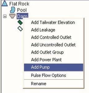To add a Pump:

Select the Dam or Outlet Group to which you want to add the Pump.
Select Add Pump from the shortcut menu (Figure 10.15) or from the component's menu in the Reservoir
Editor's menu bar.

Figure 10.15 Dam Shortcut Menu:

Add Pump

The Pump will now appear as a branch of the reservoir tree, beneath the component that it was added to.

You can rename and delete Pumps (as described in Section 10.12).

The operation of a pump is very much tied to its tailwater. Therefore, a tailwater definition is required at or above the pump in the outlet tree. See Section 10.10 for a description of adding Tailwater Elevation.

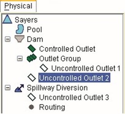10.9 Adding Uncontrolled Outlets

You can add Uncontrolled Outlets to Dams, Diverted Outlets, and Outlet Groups, as shown in Figure 10.16.

On the Physical tab, you may use either the component-specific menus in the Reservoir Editor's menu bar or the right-click shortcut menus (Figure 10.17) to add an Uncontrolled Outlet as

a component of a Dam, Diverted Outlet, or Outlet Group.

To add an Uncontrolled Outlet:

Select the Dam, Diverted Outlet, or Outlet Group to which you want to add the new Uncontrolled Outlet.
Choose Add Uncontrolled Outlet from the shortcut menu (Figure 10.17) or from the component's menu in the Reservoir Editor's menu bar.

The new Uncontrolled Outlet will Figure 10.16 Reservoir Tree:

Uncontrolled

Outlets

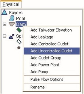
Figure 10.17 Dam Shortcut

Menu: Add

Uncontrolled

appear in the reservoir tree as a branch beneath the component you selected.

You can also rename and delete Uncontrolled Outlets in the reservoir tree, as described in Section 10.12.

Outlet

10.10 Adding Tailwater Elevation

You can add Tailwater Elevation to Dams, Diverted Outlets, and Outlet Groups, as shown in Figure 10.18.

On the Physical tab, you may use either the component-specific menus in the Reservoir Editor's menu bar or the right-click shortcut menus (Figure 10.19) to add Tailwater Elevation to a Dam, or Diverted Outlet.

To add Tailwater Elevation:

Select the Dam, Diverted Outlet, or Outlet Group to which you want to add Tailwater Elevation.
Choose Add Tailwater Elevation from the shortcut menu (Figure 10.19) or from the component's menu in the Reservoir Editor's menu bar.

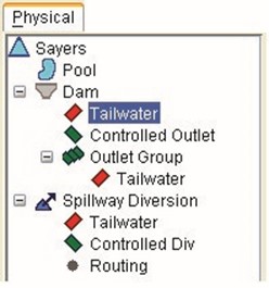
Figure 10.18 Reservoir Tree: Tailwater

Elevation

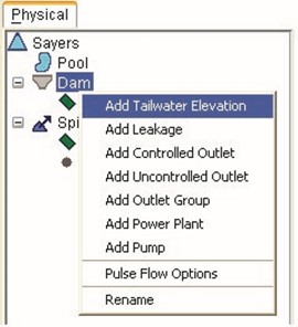
Figure 10.19 Dam Shortcut

Menu: Add

Tailwater

Elevation

The Tailwater Elevation you have added will appear in the reservoir tree as a branch beneath the component you selected.

You can also remove Tailwater Elevation from the reservoir tree, as described in Section 10.12.3.

10.11 Defining Physical Components of a Diverted Outlet

As Figure 10.20 shows, you can add

Tailwater Elevation (Section 10.10),

Outlet Groups (Section 10.7),

Controlled Outlets (Section 10.8.1),

Power Plants (Section 10.8.2),

Pumps (Section 10.8.3), and Uncontrolled Outlets (Section 10.9) to a Diverted Outlet.

Figure 10.20 Reservoir Tree:

Diverted Outlet

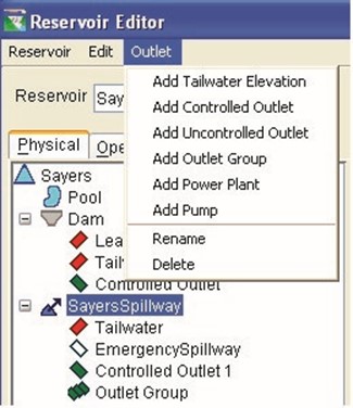On the Physical tab, you may use either the Outlet menu in the Reservoir Editor's menu bar (Figure 10.21) or the rightclick shortcut menu to specify features of a Diverted Outlet.

You can also rename and delete Diverted Outlets in the reservoir tree, as described in Section 10.12.

Figure 10.21 Reservoir Editor:

Outlet Menu for

Diverted Outlet

10.12 Renaming, Deleting, and Removing Reservoir Components

The following sections explain how to rename and delete or remove reservoir components.

10.12.1 Renaming Reservoir Components

ResSim assigns default names to reservoir components you have created in the Reservoir Network Module. You can rename Dams, Diverted Outlets, Outlet Groups, and Uncontrolled Outlets.

To rename a reservoir component:

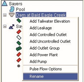Select the component by clicking on it in the reservoir tree.
Using either the right-click shortcut menu (Figure 10.22) or the component menu in the Reservoir Editor's menu bar, choose Rename. The

Rename Reservoir

Component dialog Figure 10.22 Reservoir Component box will open Shortcut Menu:

(Figure 10.23). Rename Component

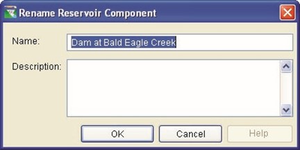
Figure 10.23 Rename Reservoir Component

Type the new name for the component in the Name field. You may also enter a new description in the Description field.
Click OK to close the dialog box. The new name will appear in the reservoir tree.

10.12.2 Deleting Reservoir Components

When you delete components from the reservoir tree, you permanently remove them from the reservoir network. You can delete Outlet Groups, Diverted Outlets, Controlled Outlets, Power Plants, Pumps, and Uncontrolled Outlets.

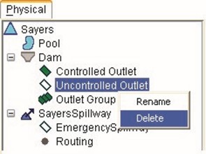To delete a reservoir component:

Select the component by clicking on it in the reservoir tree.
Using either the right-click shortcut menu (Figure 10.24) or the component
menu in the Reservoir

Editor's menu bar, choose

Delete.

3. A confirmation window will appear (Figure 10.25). Click Yes to verify the deletion.

Figure 10.24 Reservoir Component Shortcut Menu:

Delete Component

Figure 10.25 Confirm Deletion of Reservoir Component

When you delete a reservoir component, it will no longer appear in the reservoir tree.

Additionally, when you delete a Diverted Outlet, it will no longer appear in the map display of the Reservoir Network Module. To replace a Diverted Outlet, you will need to re-draw it in the map display area.

10.12.3 Removing Reservoir Parameters

You may remove Dam Leakage, Pool Evaporation and Seepage, and Tailwater Elevation from the reservoir tree without losing the associated data.

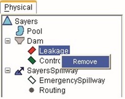To remove these parameters:

Select the parameter by clicking on it in the reservoir tree.
Using either the right-click shortcut menu (Figure
10.26) or the primary

component's menu in the

Reservoir Editor's menu Figure 10.26 Reservoir bar, choose Remove. Parameter Shortcut Menu:

Remove Parameter

A confirmation window will appear (Figure 10.27). Click Yes to verify the removal.

Figure 10.27 Confirm Removal of Reservoir

Parameter

The parameter you have removed will no longer appear in the reservoir tree. However, if you re-add this parameter, the previously entered values will be restored.

Editing Reservoir Physical Data

To edit the physical data associated with a reservoir component, select the component in the reservoir tree in the Reservoir Editor. The appropriate data editor will appear in the area to the right of the reservoir tree.

In most cases, you will want to copy and paste tabular data from a spreadsheet application into the data editors, rather than typing the data manually.

Editing Pool Physical Data

To edit physical data for a reservoir Pool, select the Pool in the reservoir tree.

Figure 10.28 shows the Reservoir Editor's Pool data editor. The table in this Editor allows you to choose either Linear or Conic Interpolation and enter the Elevation vs. Storage vs. Area data. Two plots visually represent Storage and Area values in relation to Elevation.

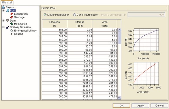
Figure 10.28 Reservoir Editor: Physical Data -- Pool

To enter data into the table, either copy and paste it from a spreadsheet application or type in the data manually.

Linear Interpolation: By default, the interpolation method ResSim uses to compute values for elevations and storages between those specified in the table is linear.
Conic Interpolation: The pool definition detailed in the regulation manual for most reservoirs was originally developed using the assumption that the volume of water between two elevations can be described by the same equation as that used to compute the volume of a section of a cone. The area of the pool surface at each elevation can be computed based on the topography of the land and the change in elevation. Using this information, ResSim can compute the storage between the two elevations. This method of computing storage is available with the conic interpolation option. This option requires you to input an elevation vs. area relationship and a starting storage value at the lowest elevation in the table. ResSim will then compute the storage values using the conic assumption. Conic interpolation will also be used to obtain intermediate storage values for elevations between those explicitly entered in the table.

The following are requirements for Elevation, Storage, and Area data:

You must enter at least two rows, with values increasing down the columns.
You may not enter duplicate values.
The maximum elevation should not exceed the Elevation at top of Dam.

Be sure to click the Apply button before moving on to edit the next component.

10.14.1 Editing Pool Evaporation Data

To edit Evaporation data, select Evaporation in the reservoir tree. Figure 10.29 shows the Reservoir Editor's Evaporation data editor and its corresponding mini-plot. The mini-plot will reflect the values you enter and can be viewed in full size when you double-click on it.

You may choose either Monthly Average Evaporation or Evaporation Time-Series data.

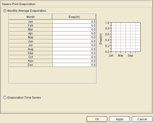
Figure 10.29 Reservoir Editor: Physical Data -- Pool

Evaporation

Monthly Average Evaporation: Enter Evaporation values by month. To enter data into the table, either copy and paste it from a spreadsheet application or type in the values manually.
Evaporation Time Series: If you select this option, you will need to specify the time-series data source when you create an Alternative (Chapter 13).

Be sure to click the Apply button before moving on to edit the next component.

10.14.2 Editing Pool Seepage

To edit Seepage data, select Seepage in the reservoir tree. Figure 10.30 shows the Reservoir Editor's Seepage data editor and its corresponding mini-plot. The mini-plot will reflect the values you enter and can be viewed in full size when you double-click on it.

You may choose either Constant Seepage or Seepage as a function of Reservoir Elevation.

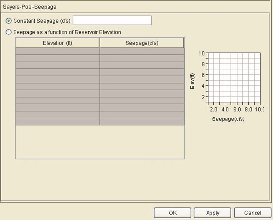
Figure 10.30 Reservoir Editor: Physical Data -- Pool Seepage

Constant Seepage: Enter the constant value in the field provided.
Seepage as a Function of Reservoir Elevation: Enter Elevation and Seepage values into the table. To enter data into the table, either copy and paste it from a spreadsheet application or type in the values manually.

Be sure to click the Apply button before moving on to edit the next component.

10.15 Editing Dam Leakage

To edit Leakage data for a dam, select Leakage in the reservoir tree. Figure 10.31 shows the Reservoir Editor's Leakage data editor and its corresponding mini-plot. The mini-plot will reflect the values you enter and can be viewed in full size when you double-click on it.

The Leakage data editor allows you to define Leakage as a function of pool Elevation. Leakage, although referred to as a "loss," is not a true loss of flow to the system. In fact, leakage effectively passes through the dam into the downstream system at the downstream (or tailwater) junction.

Figure 10.31 Reservoir Editor: Physical Data -- Dam Leakage

To enter data into the table, either copy and paste it from a spreadsheet application or type in the data manually.

Be sure to click the Apply button before moving on to edit the next component.

10.16 Editing Controlled Outlet Physical Data

A Controlled Outlet can be a component of a Dam, Diverted Outlet, or Outlet Group. Additionally, a Controlled Outlet may have its own Tailwater Elevation.

To edit data for the primary Controlled Outlet, select the name of the Controlled Outlet in the reservoir tree.

Figure 10.32 shows the Reservoir Editor's Controlled Outlet data editor and its corresponding mini-plot. The mini-plot will reflect the values you enter and can be viewed in full size when you double-click on it.

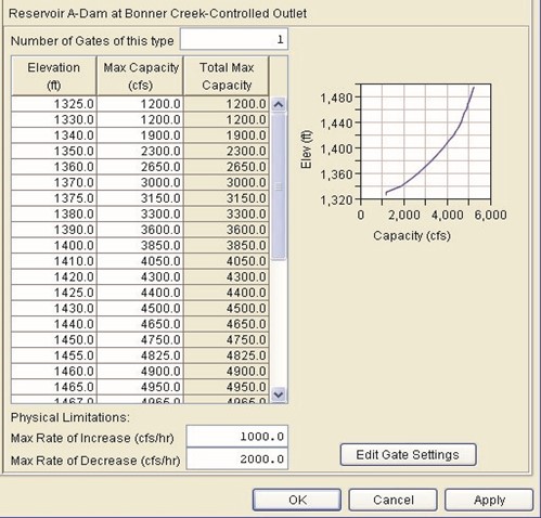
Figure 10.32 Controlled Outlet (no Gate Settings)

To enter Controlled Outlet data:

Specify the Number of Gates of this type.
Enter Elevation and corresponding Max Capacity flow values into the table. Max Capacity values reflect the maximum physical flow constraint per gate of the outlet at the corresponding elevation. You can either copy and paste data from a spreadsheet application or type in the values manually. Total Max Capacity will automatically be calculated as the product of the Max Capacity times the number of gates.
Optionally, specify Physical Limitations for Max Rate of Increase and Max Rate of Decrease.

Click the Edit Gate Settings button to access the Gate Settings dialog box (Figure 10.33). Gate settings are sometimes known as "cranks." 5. Choose either Specify
Maximum Capacity Only or Specify Capacity at Specific Gate Openings. To Specify Capacity at Specific Gate Openings:

Select the Number of

Gate Settings (or

"cranks") and the Gate Setting Units (Length or Percent).

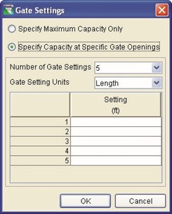
Figure 10.33 Gate Settings

Enter the Setting for each gate.

6. Click OK to close the Gate Settings dialog box.

Note: Even though you can enter the appropriate Gate Settings, ResSim does not currently make use of this information in its operations. It will, however, produce a time series of gate settings as output based on the final release from the outlet.

Figure 10.34 shows the Reservoir Editor's Controlled Outlet data editor with Gate Settings specified.

Figure 10.34 Controlled Outlet (with Gate Settings)

When you are done entering Controlled Outlet data, be sure to click the Apply button before moving on to edit the next component.

10.17 Editing Power Plant Physical Data

A Power Plant can be a component of a Dam, Diverted Outlet, or Outlet Group. To edit data for a Power Plant, select the Power Plant in the reservoir tree.

The Reservoir Editor's Power Plant data editor has five tabs that allow you to edit data for Outlet Capacity, Plant Capacity, Efficiency, Station Use, and Hydraulic Losses, as described in the following sections.

10.17.1 Editing Outlet Capacity Data for a Power Plant

On the Outlet tab (Figure 10.35), you will enter the rating table for the physical capacity of this outlet. You can also specify the increasing and decreasing physical limitations (i.e., physical rate-ofchange constraints).

To enter Outlet data:

Specify the Number of Gates of this type.
Enter Elevation and corresponding Max Capacity flow values (per gate) into the table. You can either copy and paste data from a spreadsheet application or type in the values manually.
Optionally, specify Physical Limitations for Max Rate of Increase and Max Rate of Decrease.

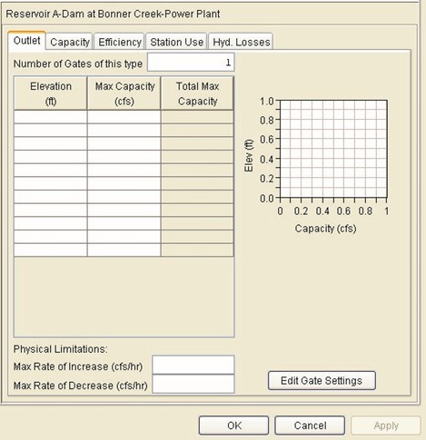
Figure 10.35 Power Plant Physical Data Editor: Outlet Tab

10.17.2 Editing Capacity Data for a Power Plant

On the Capacity tab (Figure 10.36), you can enter values for the Installed Capacity and an Overload Factor, and you can select one of five options for the Variable Capacity.

Figure 10.36 Power Plant Physical Data Editor: Capacity Tab

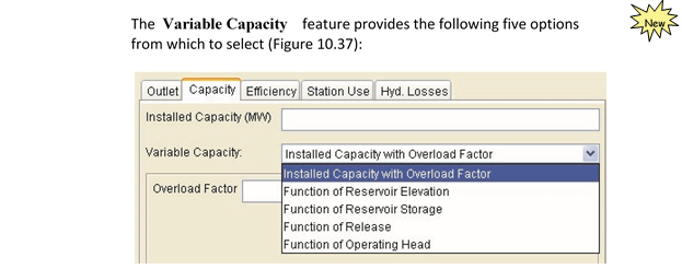
Figure 10.37 Power Plant Capacity Tab: Variable Capacity Options

Installed Capacity with Overload Factor option (previously shown in Figure 10.36): The Installed Capacity is entered in megawatts (MW) and represents the nameplate capacity for the power plant. The Overload Factor is used as a multiplier for the Installed Capacity to determine the maximum energy the power plant can produce in a time interval. To use the full Installed Capacity, enter an Overload Factor of 1.0. For example, to overload a plant's installed capacity by 10%, enter a factor of 1.10.
Function of Reservoir Elevation option (Figure 10.38): In addition to entering the Installed Capacity value, you should insert the appropriate number of rows in the Elevation vs. Capacity table and then enter the function relationship values.

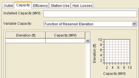
Figure 10.38 Power Plant Capacity Tab:

Variable Capacity -- Function of Reservoir Elevation

Function of Reservoir Storage option (Figure 10.39): In addition to entering the Installed Capacity value, you should insert the appropriate number of rows in the Storage vs. Capacity table and then enter the function relationship values.

Figure 10.39 Power Plant Capacity Tab:

Variable Capacity -- Function of Reservoir Storage

Function of Release option (Figure 10.40): In addition to entering the Installed Capacity value, you should insert the appropriate number of rows in the Release vs. Capacity table and then enter the function relationship values.

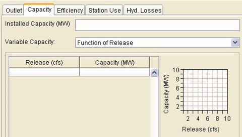
Figure 10.40 Power Plant Capacity Tab:

Variable Capacity -- Function of Release

Function of Operating Head option (Figure 10.41): In addition to entering the Installed Capacity value, you should insert the appropriate number of rows in the Head vs. Capacity table and then enter the function relationship values.

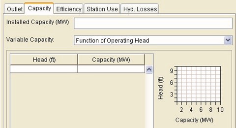
Figure 10.41 Power Plant Capacity Tab:

Variable Capacity -- Function of Operating Head

10.17.3 Editing Efficiency Data for a Power Plant

Power efficiency is the total efficiency (generator efficiency x turbine efficiency) of the power plant. On the Efficiency tab, you can specify an Efficiency Method from a list of four options: Constant, Function of Reservoir Elevation, Function of Release, or Function of Operating Head. Each Efficiency Method has its own data editor, as described in the following sections.

10.17.3.1 Constant Efficiency Method

For the Constant Efficiency method (Figure 10.42), enter a constant percentage value for the overall, generator plus turbine, plant efficiency (typical plant efficiency ranges between 80% and 90%). In actual operation, however, the turbine-generator efficiency varies throughout its range of operation (subsequent sections describe efficiency as a function of elevation, release or operating head).

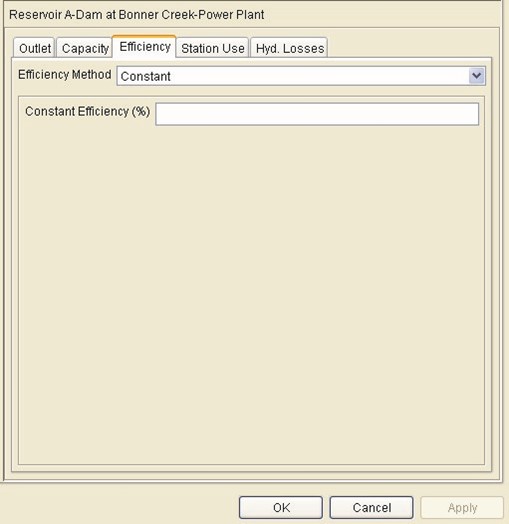
Figure 10.42 Power Plant Physical Data Editor:

Efficiency Tab -- Constant Efficiency Method

When you have finished entering Efficiency data, be sure to click the Apply button before moving on to the next tab.

10.17.3.2 Function of Reservoir Elevation Efficiency Method

For the Function of Reservoir Elevation efficiency method (Figure 10.43), enter values for Elevation and Efficiency. The mini-plot will reflect the values you enter and can be viewed in full size when you double-click on it.

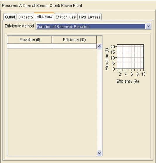
Figure 10.43 Power Plant Physical Data Editor:

Efficiency Tab -- Function of Reservoir Elevation

When you have finished entering Efficiency data, be sure to click the Apply button before moving on to the next tab.

10.17.3.3 Function of Release Efficiency Method

For the Function of Release efficiency method (Figure 10.44), enter values for Release and Efficiency. The mini-plot will reflect the values you enter and can be viewed in full size when you double-click on it.

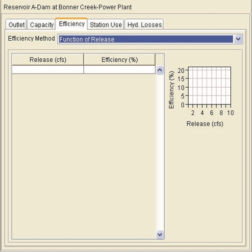
Figure 10.44 Power Plant Physical Data Editor:

Efficiency Tab -- Function of Release

When you have finished entering Efficiency data, be sure to click the Apply button before moving on to the next tab.

10.17.3.4 Function of Operating Head Efficiency Method

For the Function of Operating Head efficiency method (Figure 10.45), enter values for Head and Efficiency. The mini-plot will reflect the values you enter and can be viewed in full size when you double-click on it.

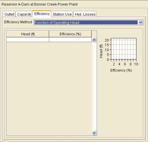
Figure 10.45 Power Plant Physical Data Editor:

Efficiency Tab -- Function of Operating Head

When you have finished entering Efficiency data, be sure to click the Apply button before moving on to the next tab.

10.17.4 Editing Station Use Data for a Power Plant

Station Use is a portion of the flow that passes through the outlet but is not used to generate power for the "grid." On the Station Use tab, you can define the Station Use Method as Constant or as a Function of Release. Each method has its own data editor, as described in the following sections.

10.17.4.1 Constant Station Use Method

The Constant station use method (Figure 10.46) simply means that the flow "loss" is not affected by any parameter.

Enter a value for Constant Station Use.

Figure 10.46 Power Plant Physical Data Editor:

Station Use Tab -- Constant Method

When you have finished entering Station Use data, be sure to click the Apply button before moving on to the next tab.

10.17.4.2 Function of Release Station Use Method

The loss of flow for generating hydropower through station use can also be defined as a function of flow entering the outlet. For the Function of Release station use method (Figure 10.47), enter values for Release (flow) and Use (the loss in flow units). The mini-plot will reflect the values you enter and can be viewed in full size when you double-click on it.

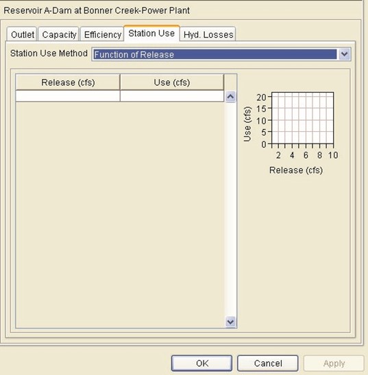
Figure 10.47 Power Plant Physical Data Editor:

Station Use Tab -- Function of Release Method

When you have finished entering Station Use data, be sure to click the Apply button before moving on to the next tab.

10.17.5 Editing Hydraulic Losses Data for a Power Plant

Hydraulic loss can also be referred to as head loss. ResSim uses the value of head (the difference between the pool elevation and the tailwater elevation) within the power equations to compute capacity. When you enter a hydraulic loss, you are describing a loss to the head, thereby reducing the plant's generating capacity.

You can choose one of two methods to describe hydraulic losses. On the Hydraulic Losses tab, you can specify the head loss as a Constant or as a Function of Release (flow through the outlet). Each method has its own data editor, as described in the following sections.

10.17.5.1 Constant Hydraulic Losses Method

For the Constant hydraulic losses method (Figure 10.48), enter a value for Constant Hydraulic Loss.

Figure 10.48 Power Plant Physical Data Editor:

Hydraulic Losses Tab -- Constant Method

When you have finished entering Hydraulic Losses data, be sure to click the Apply button before moving on.

10.17.5.2 Function of Release Hydraulic Losses Method

For the Function of Release hydraulic losses method (Figure 10.49), enter values for Release and Loss to describe the head loss as a function of flow through the outlet. The mini-plot will reflect the values you enter and can be viewed in full size when you double-click on it.

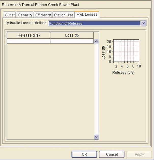
Figure 10.49 Power Plant Physical Data Editor:

Hydraulic Losses Tab -- Function of Release Method

Release: Flow through the outlet.
Loss: Head Loss, a unit of length to be removed from the head value used to compute generating capacity.

When you have finished entering Hydraulic Losses data, be sure to click the Apply button before moving on.

10.18 Editing Pump Physical Data

A Pump can be a component of a Dam, Diverted Outlet, or Outlet Group.

In the Pump editor, you can define the Pump Capacity as Constant or as a Function of Operating Head. Each method has its own data editor, as described in the following sections.

10.18.1 Pump Capacity as Constant

The Constant Pump Capacity method (Figure 10.50) simply means that the maximum capacity of the pump is not affected by any other parameter.

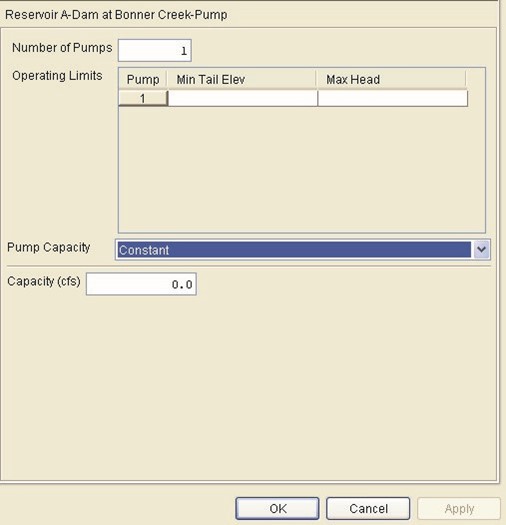
Figure 10.50 Pump Physical Data Editor:

Pump Capacity -- Constant

Enter the Number of Pumps associated with this pump outlet.
For each pump, enter the Minimum Tailwater Elevation and corresponding Maximum Head.
Select Constant for Pump Capacity.
Enter a value for the Capacity.

When you have finished entering Pump data, be sure to click the Apply button before moving on to the next component.

10.18.2 Pump Capacity as Function of Operating Head

The Pump Capacity can be specified as a Function of Operating Head (Figure 10.51).

Figure 10.51 Pump Physical Data Editor:

Pump Capacity -- Function of Operating Head

Enter the Number of Pumps associated with this pump outlet.
For each pump, enter the Minimum Tailwater Elevation and corresponding Maximum Head.
Select Function of Operating Head for Pump Capacity.
Enter into the table the values for Operating Head and corresponding values of Pump Capacity.

When you have finished entering Pump data, be sure to click the Apply button before moving on to the next component.

10.19 Editing Uncontrolled Outlet Physical Data

An Uncontrolled Outlet can be a component of a Dam, Diverted Outlet, or Outlet Group. The uncontrolled outlet is an uncontrolled spillway and you can use a weir equation to compute the flow over the spillway. Otherwise, the outlet can be defined by a simple rating curve that describes flow through the outlet.

Figure 10.52 shows the Reservoir Editor's Uncontrolled Outlet data editor and its corresponding mini-plot. The mini-plot will reflect the values you enter and can be viewed in full size when you double-click on it.

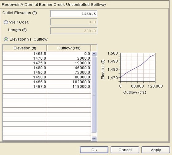
Figure 10.52 Reservoir Editor: Physical Data -- Uncontrolled Outlet

In the Uncontrolled Spillway data editor you will specify Outlet Elevation. This elevation will serve as a trigger to determine when this outlet starts "flowing." Next, choose how you want to represent your uncontrolled outlet: as a spillway using the weir equation (Weir Coefficient) or as a rating curve (Elevation vs. Outflow). If you choose to define your uncontrolled outlet as a spillway, enter the spillway length and weir coefficient; otherwise, enter the rating curve's elevation and outflow values.

Outlet Elevation: Minimum elevation at which the outlet will begin to release water.
Weir Coefficient: Typically in the range 2.6-4.0 depending on the shape of the spillway crest. This value determines flow over the spillway in the weir equation.
Length: Spillway length.

Elevation vs. Outflow: To enter data into the table, either copy and paste it from a spreadsheet application or type in the data manually.

Be sure to click the Apply button before moving on to edit the next component.

10.20 Editing Tailwater Elevation Physical Data

Tailwater Elevation can be a component of a Dam, Diverted Outlet, Outlet Group, Controlled Outlet, Power Plant, and Pump. If you have defined one or more power plants for this reservoir, you must add a Tailwater elevation so the head can be computed for the power computations. Three different methods for defining tailwater are available. If you define more than one, ResSim will compute all defined but will use only the highest to determine the head.

To edit Tailwater Elevation data, select the Tailwater component in the reservoir tree. Figure 10.53 shows the Reservoir Editor's Tailwater Elevation data editor. The mini-plot will reflect the rating curve values you enter and can be viewed in full size when you double-click on it.

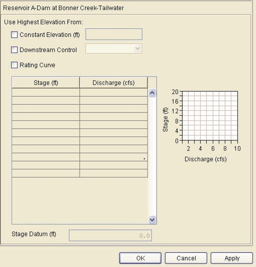
Figure 10.53 Reservoir Editor: Physical Data -- Tailwater

Constant Elevation: Enter a value for the tailwater elevation. If the reservoir has a stilling basin at the tailwater, a constant elevation may be an appropriate definition.
Downstream Control: Select a location from the list. This list will only contain downstream reservoirs or downstream junctions (where a rating curve has been specified so the elevation of the junction can be determined).
Rating Curve: You can also apply a rating curve to represent the tailwater of the dam or outlet of the reservoir. You may either copy and paste the data from a spreadsheet application or type in the values manually.
- Stage: The height from some datum, representing the water surface elevation.
- Discharge: The flow passing that location that would produce the associated water surface elevation.

Stage Datum: The "zero" elevation against which stage is measured. This elevation must be in the same vertical reference as the elevations describing the reservoir.

Be sure to click the Apply button before moving on to edit the next component.

10.21 Viewing Composite Release Capacity Tables

Composite Release Capacity tables and their corresponding mini-plots provide a summary of outlet capacity data for Controlled and Uncontrolled Outlets of a reservoir. Figure 10.54 shows a Composite Release Capacity table for a reservoir. The mini-plot reflects the composite values and can be viewed in full size when you double-click on it.

Figure 10.54 Composite Release Capacity Table

Composite Release Capacity tables are informational and are not editable. Instead, they fill in automatically as you add data for the individual components.

Reservoir Composite Release Capacity Table

To view the Reservoir Composite Release Capacity table, select the

Reservoir's name at the top of the reservoir tree (corresponding to the symbol) as shown in Figure 10.49.

In ResSim, a reservoir consists of, minimally, a Pool and a Dam; it may also include Diverted Outlets. The dam (and diverted outlet) can then, in turn, include outlets and outlet groups. The dam, diverted outlet, and any outlet group will display Composite Release Capacity tables similar to that of the reservoir to represent the total outlet capacity of the components contained within each group.

Dam Composite Release Capacity Table

To access the Dam Release Capacity table, select the Dam in the reservoir tree (corresponding to thesymbol).

The components of a dam that influence the Composite Release Capacity table include controlled outlets, uncontrolled outlets, and outlet groups.

Diverted Outlet Composite Release Capacity Table

To access the Diverted Outlet Composite Release Capacity table, select the Diverted Outlet in the reservoir tree (corresponding to the symbol).

The components of a diverted outlet that influence the composite release capacity table include controlled outlets, uncontrolled outlets, and outlet groups.

Outlet Group Composite Release Capacity Table

To access the Outlet Group Composite Release Capacity table, select the Outlet Group in the reservoir tree (corresponding to the symbol).

An outlet group can be a component of a dam, diverted outlet, or another outlet group. The components that can influence the Outlet Group Composite Release Capacity table include controlled outlets, uncontrolled outlets, and outlet groups.

10.22 Reservoir Editor: Pulse Flow Options

From the Reservoir editor's Physical tab, an advanced option is available to redefine the pulse flow that is used in the ResSim flow routing computations associated with reservoir release determinations for downstream operations. A value of 5000 cfs (142 cms) is used by default. However, by selecting the Pulse Flow Options available from the Dam's shortcut menu (Figure 10.55) or the Dam menu in the Reservoir Editor's menu bar, you can set the value more appropriately for the range of flows expected in your river system (Figure 10.56).

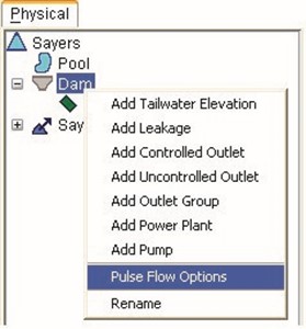
Figure 10.55 Reservoir Tree:

Dam Shortcut Menu, Pulse Flow Options

Figure 10.56 Dam Component:

Pulse Routing Options Editor

10.23 Reservoir Editor: Observed Data Tab

Use the Observed Data tab (Figure 10.57) to indicate that observed data is available for comparison purposes. If the Observed box in the table is checked, then there will be a corresponding entry in the Observed TimeSeries mapping table when you create an Alternative (Chapter 13).

Figure 10.57 Reservoir Editor: Observed Data Tab

To edit another reservoir without exiting the Reservoir Editor, click the Apply button and then select another reservoir from the Reservoir name list or use the navigator buttons.

Chapter 11

Defining Reservoir Operations Data

Section Page

11 DEFINING RESERVOIR OPERATIONS DATA .......................................................1 1-1

11.1 RESERVOIR EDITOR'S OPERATIONS TAB ...........................................................1 1-2 11.2 RESERVOIR OPERATION SETS .........................................................................1 1-3

11.2.1 CREATING A NEW OPERATION SET ......................................................1 1-3 11.2.2 RENAMING AN OPERATION SET ...........................................................1 1-4 11.2.3 COPYING AN OPERATION SET .............................................................1 1-5 11.2.4 DELETING AN OPERATION SET ............................................................1 1-5 11.2.5 EDITING AN OPERATION SET ...............................................................1 1-6

11.3 RESERVOIR OPERATION ZONES .......................................................................1 1-6

11.3.1 RENAMING AND DESCRIBING OPERATION ZONES ................................. 11-7 11.3.2 ADDING A NEW RESERVOIR STORAGE ZONE ........................................1 1-7 11.3.3 DEFINING OPERATION ZONES .............................................................1 1-8 11.3.4 DELETING OPERATION ZONES ...........................................................1 1-13

11.4 UNDERSTANDING RESERVOIR OPERATION RULES ........................................... 11-14

11.4.1 RELEASE DECISION PROCESS ...........................................................1 1-14 11.4.2 USING EXISTING RULES ....................................................................1 1-14 11.4.3 REMOVING RULES ............................................................................1 1-15 11.4.4 DELETING RULES .............................................................................1 1-15 11.4.5 PRIORITIZING RULES ........................................................................1 1-15 11.4.6 RENAMING RULES ............................................................................1 1-15

11.5 DEFINING RESERVOIR OPERATION RULES ...................................................... 11-16

11.5.1 ADDING A NEW OPERATION RULE TO A ZONE ..................................... 11-17 11.5.2 ADDING AN EXISTING RULE TO A ZONE .............................................. 11-18 11.5.3 DEFINING A RELEASE FUNCTION RULE .............................................. 11-19 11.5.4 DEFINING A DOWNSTREAM CONTROL FUNCTION RULE ....................... 11-25 11.5.5 DEFINING A TANDEM OPERATION RULE ............................................. 11-30 11.5.6 DEFINING AN INDUCED SURCHARGE RULE ......................................... 11-32 11.5.7 DEFINING A FLOW RATE OF CHANGE LIMIT RULE ................................ 11-42 11.5.8 DEFINING AN ELEVATION RATE OF CHANGE LIMIT RULE ...................... 11-43 11.5.9 DEFINING HYDROPOWER RULES ....................................................... 11-44 11.5.10 DEFINING A PUMP SCHEDULE RULE................................................... 11-58 11.5.11 DEFINING SCRIPTED RULES ..............................................................1 1-62 11.5.12 DEFINING IF_BLOCKS .......................................................................1 1-68

11.6 COMMON OPTIONS FOR RULE DEFINITION ...................................................... 11-74

11.6.1 INTERPOLATION METHOD ..................................................................1 1-74 11.6.2 PERIOD AVERAGE LIMIT ....................................................................1 1-75 11.6.3 HOUR OF DAY MULTIPLIER ................................................................1 1-77 11.6.4 DAY OF WEEK MULTIPLIER................................................................1 1-78 11.6.5 RISING / FALLING CONDITION ............................................................ 11-79 11.6.6 SEASONAL VARIATION ......................................................................1 1-80

11.7 SELECTING THE RESERVOIR GUIDE CURVE .................................................... 11-82 11.8 SPECIFYING RELEASE ALLOCATION ................................................................1 1-82 11.9 DEFINING OUTAGE SCHEDULE .......................................................................1 1-86

11.10 ADJUSTING THE GUIDE CURVE BASED ON FLOOD CONTROL STORAGE CREDIT .... 11-88

11.11 EDITING THE RESERVOIR DECISION SCHEDULE ............................................... 11-92 11.12 PROJECTED ELEVATION .................................................................................1 1 New -93 11.13 STATE VARIABLES .........................................................................................1 1-95

11.13.1 INTERNAL STATE VARIABLES (MODEL VARIABLES).............................. 11-96

11.13.2 USER-DEFINED STATE VARIABLES .................................................... 11-96 11.13.3 DEVELOPMENT CONCEPTS FOR STATE VARIABLES ............................. 11-96

11.13.4 CREATING AND EDITING STATE VARIABLE SCRIPTS ............................ 11-97

11.14 IMPORTING ELEMENT PROPERTIES ............................................................... 11-103

List of Figures

Figure
Number	Page
FIGURE 11.1	RESERVOIR EDITOR OPERATIONS TAB........................................................1 1-2
FIGURE 11.2	NEW OPERATION SET ................................................................................1 1-4
FIGURE 11.3	RENAME OPERATION SET ..........................................................................1 1-4
FIGURE 11.4	DUPLICATE OPERATION SET ......................................................................1 1-5
FIGURE 11.5	SELECT OPERATION SET TO DELETE ..........................................................1 1-5
FIGURE 11.6	RESERVOIR EDITOR SHOWING NEW OPERATION SET ..................................1 1-6
FIGURE 11.7	NEW ZONE ................................................................................................1 1-7
FIGURE 11.8	RESERVOIR EDITOR--OPERATIONS TAB: ZONE EDITOR ...............................1 1-8

FIGURE 11.9 INDEPENDENT VARIABLE DEFINITION:

New

"ZONE IS A FUNCTION OF:" SELECTION ........................................................ 11-9

New

FIGURE 11.10 FLEXIBLE ZONE DEFINITION – DATE AND TIME .............................................1 1-9 FIGURE 11.11 FLEXIBLE ZONE DEFINITION – MODEL VARIABLE ........................................ 11-10 ^NewFIGURE 11.12 TIME SERIES OPTIONS FOR FLEXIBLE ZONE DEFINITION ............................ 11-10 ^NewFIGURE 11.13 FLEXIBLE ZONE DEFINITION – MODEL VARIABLE RELATIONSHIP TABLE DEFINITION ...............................................................................1 1-11 FIGURE 11.14 FLEXIBLE ZONE DEFINITION – EXTERNAL VARIABLE ................................... 11-11 ^New

New

FIGURE 11.15 FLEXIBLE ZONE DEFINITION – EXTERNAL VARIABLE RELATIONSHIP

TABLE DEFINITION ..............................................................................1 1^New-12 FIGURE 11.16 FLEXIBLE ZONE DEFINITION – STATE VARIABLE ......................................... 11-12 ^New

FIGURE 11.17 FLEXIBLE ZONE DEFINITION – STATE VARIABLE RELATIONSHIP

TABLE DEFINITION ..............................................................................1 1^New-13

FIGURE 11.18	NEW OPERATING RULE ............................................................................1 1-17
FIGURE 11.19	SELECT EXISTING RULE ...........................................................................1 1-18
FIGURE 11.20	RESERVOIR EDITOR--OPERATIONS TAB: NEW RELEASE FUNCTION RULE ... 11-20
FIGURE 11.21	RELEASE FUNCTION RULE, SELECTING A FUNCTION FROM

INDEPENDENT VARIABLE DEFINITION EDITOR ....................................... 11-20

FIGURE 11.22 RELEASE FUNCTION RULE, SELECT AN INDEPENDENT VARIABLE FROM

THE MODEL VARIABLE LIST ................................................................. 11-21

FIGURE 11.23 RELEASE FUNCTION RULE, DEFINING AN EXTERNAL VARIABLE AS

THE INDEPENDENT VARIABLE ..............................................................1 1-21

FIGURE 11.24 RELEASE FUNCTION RULE, SELECT A STATE VARIABLE AS

THE INDEPENDENT VARIABLE ..............................................................1 1-22

FIGURE 11.25	TIME SERIES OPTIONS FOR MODEL, EXTERNAL, AND STATE VARIABLES ..... 11-22
FIGURE 11.26	EXAMPLE OF COMPLETED RELEASE FUNCTION RULE ................................ 11-24
FIGURE 11.27	RESERVOIR EDITOR--NEW OPERATING RULE:

DOWNSTREAM CONTROL FUNCTION ................................................... 11-25

FIGURE 11.28 RESERVOIR EDITOR--EXAMPLE OF A DOWNSTREAM CONTROL

FUNCTION RULE ................................................................................1 1-26

11.29 FLOW CONTINGENCY FOR DOWNSTREAM OPERATION ............................... 11-27 ^New

11.30 ADVANCED OPTIONS FOR DOWNSTREAM RULE(S) – _New

GLOBAL OPTIONS ...............................................................................1 1-28

FIGURE 11.31 ADVANCED OPTIONS FOR DOWNSTREAM RULE –

New

RULE SPECIFIC OPTIONS ....................................................................1 1-28

FIGURE 11.32 RESERVOIR EDITOR--NEW OPERATING RULE: TANDEM OPERATION .......... 11-30 FIGURE 11.33 RESERVOIR EDITOR--EXAMPLE OF A TANDEM OPERATION RULE ................ 11-31

FIGURE 11.34 RESERVOIR EDITOR--OPERATIONS TAB:

CREATE INDUCED SURCHARGE RULE .................................................. 11-32

FIGURE 11.35 INDUCED SURCHARGE RULE EDITOR, USE

INDUCED SURCHARGE FUNCTION OPTION ............................................ 11-33

FIGURE 11.36 INDUCED SURCHARGE RULE EDITOR, COMPLETED EXAMPLE OF

INDUCED SURCHARGE FUNCTION ........................................................1 1-34

FIGURE 11.37 PLOT OF COMPUTED INDUCED SURCHARGE CURVES

(WITH THE DISCHARGE CAPACITY CURVE) ........................................... 11-35

FIGURE 11.38 OPTIONS MENU (FROM INDUCED SURCHARGE CURVES PLOT) ................... 11-35 FIGURE 11.39 EDIT INFLOW FOR CURVES… (FROM OPTIONS MENU OF

INDUCED SURCHARGE CURVES PLOT) ................................................. 11-35

FIGURE 11.40 PLOT OF COMPUTED INDUCED SURCHARGE CURVES

(WITHOUT THE DISCHARGE CAPACITY CURVE) ..................................... 11-36

FIGURE 11.41 INDUCED SURCHARGE RULE EDITOR, SPECIFY THE

ESRD CURVES OPTION ......................................................................1 1^New-37

FIGURE 11.42 INDUCED SURCHARGE RULE – ENTERING ESRD VALUES

(INFLOWS OR RATE OF RISE) ..............................................................1 ^New1-38

FIGURE 11.43 INDUCED SURCHARGE RULE EDITOR, COMPLETED EXAMPLE OF

SPECIFYING THE ESRD CURVES .........................................................1 1^New-38

FIGURE 11.44 PLOT OF INDUCED SURCHARGE CURVES FOR SPECIFIED

New

ESRD INFLOW VALUES ......................................................................1 1-39

FIGURE 11.45 INDUCED SURCHARGE -- FALLING POOL OPTIONS ..................................... 11-40 FIGURE 11.46 INDUCED SURCHARGE -- INFLOW TIME SERIES OPTIONS ............................ 11-41

FIGURE 11.47 RESERVOIR EDITOR--OPERATIONS TAB:

FLOW RATE OF CHANGE LIMIT RULE ................................................... 11-42

FIGURE 11.48 RESERVOIR EDITOR--OPERATIONS TAB:

ELEVATION RATE OF CHANGE LIMIT RULE (POOL) ................................ 11-43

FIGURE 11.49	HYDROPOWER RULE TYPES .....................................................................1 1-44
FIGURE 11.50	HYDROPOWER – SCHEDULE RULE EDITOR ................................................ 11-45
FIGURE 11.51	POWER GENERATION REQUIREMENT OPTION ........................................... 11-46
FIGURE 11.52	HYDROPOWER – TIME SERIES REQUIREMENT RULE EDITOR ...................... 11-47
FIGURE 11.53	HYDROPOWER – POWER GUIDE CURVE RULE EDITOR ............................... 11-48
FIGURE 11.54	HYDROPOWER – SYSTEM SCHEDULE RULE EDITOR .................................. 11-50
FIGURE 11.55	HYDROPOWER SYSTEM RULE: RESERVOIR LIST EDITOR ........................... 11-50
FIGURE 11.56	POWER GENERATION PATTERN (ALL WEEK) ............................................. 11-52
FIGURE 11.57	POWER GENERATION PATTERN (WEEKDAYS & WEEKENDS) ....................... 11-52
FIGURE 11.58	POWER GENERATION PATTERN (EACH DAY) ............................................. 11-53

11.59 POWER REQUIREMENT ALL HOURS OF THE DAY (DEFAULT VALUE = 1.0) .... 11-54

11.60 POWER REQUIREMENT PORTION OF THE DAY (8 A.M. TO 5 P.M.) ................ 11-54

FIGURE 11.61 HOUR OF DAY WEIGHTING TO "DOUBLE" THE POWER REQUIREMENT

FOR PORTION OF DAY ........................................................................1 1-55

FIGURE 11.62 WEIGHTING FACTORS THROUGHOUT THE DAYS OF THE WEEK ................... 11-56 FIGURE 11.63 DEFINITION OF SEASONAL VARIATION FOR POWER GENERATION PATTERN . 11-57

FIGURE 11.64 SELECTION OF SEASONS FOR SEASONAL VARIATION FOR

POWER GENERATION PATTERN ..........................................................1 1-57

FIGURE 11.65	NEW OPERATING RULE: PUMP SCHEDULE ............................................... 11-58
FIGURE 11.66	PUMP RULE EDITOR ................................................................................1 1-58
FIGURE 11.67	PUMP RULE EDITOR: TARGET FILL ELEVATION OPTION IS "CONSTANT" ....... 11-59
FIGURE 11.68	PUMP RULE EDITOR: TARGET FILL ELEVATION OPTION IS "STORAGE ZONE" 11-59
FIGURE 11.69	PUMP RULE EDITOR: TARGET FILL ELEVATION OPTION IS

"SEASONALLY VARYING" ....................................................................1 1-59

FIGURE 11.70	DAILY PUMPING PERIOD USING FIXED HOUR RANGE ................................. 11-60
FIGURE 11.71	DAILY PUMPING PERIOD USING BETWEEN SUNSET AND SUNRISE ............... 11-61
FIGURE 11.72	NEW OPERATING RULE: SCRIPT ..............................................................1 1-62
FIGURE 11.73	SCRIPTED RULE EDITOR "DEFAULT" TEMPLATE ......................................... 11-63
FIGURE 11.74	SCRIPTED RULE EDITOR – API PANE ITEM NODES AND TEXT ..................... 11-64
FIGURE 11.75	DEFAULT CODE TEMPLATE.......................................................................1 1-65
FIGURE 11.76	SCRIPTED RULE EDITOR – API PANE AND PREVIEW BAR ........................... 11-66
FIGURE 11.77	SCRIPTED RULE EDITOR – API PANE SHOWING JYTHON

DATA TYPES AND OBJECT CLASSES (WITH TOOLTIPS) ......................... 11-67

FIGURE 11.78	NEW IF_BLOCK .......................................................................................1 1-68
FIGURE 11.79	CONDITIONAL TEST EDITOR (ADD CONDITIONS TO IF_BLOCKS) ................. 11-69
FIGURE 11.80	CONDITIONAL TEST EDITOR – SELECT VALUE TYPE ................................... 11-69
FIGURE 11.81	CONDITIONAL TEST EDITOR – PICK VALUE ................................................ 11-70
FIGURE 11.82	CONDITIONAL TEST EDITOR – SELECT TIME SERIES FOR VALUE 1 .............. 11-70
FIGURE 11.83	CONDITIONAL TEST EDITOR – SELECT OPERATOR ..................................... 11-71
FIGURE 11.84	CONDITIONAL TEST EDITOR – SELECT TYPE AND DEFINE VALUE 2 ............. 11-71
FIGURE 11.85	CONDITIONAL TEST EDITOR – APPLY LABEL TO CONDITIONAL TEST ........... 11-72
FIGURE 11.86	EXAMPLE OF COMPOUND CONDITIONAL TESTS ......................................... 11-72
FIGURE 11.87	CONDITIONAL TEST SHORTCUT MENU ...................................................... 11-73
FIGURE 11.88	ADD RULE TO CONDITIONAL TEST ............................................................1 1-73
FIGURE 11.89	IF_BLOCK SHORTCUT MENU ....................................................................1 1-73
FIGURE 11.90	INTERPOLATION METHODS .......................................................................1 1-74
FIGURE 11.91	LINEAR INTERPOLATION METHOD .............................................................1 1-74
FIGURE 11.92	STEP INTERPOLATION METHOD ................................................................1 1-74
FIGURE 11.93	CUBIC INTERPOLATION METHOD ...............................................................1 1-75
FIGURE 11.94	PERIOD AVERAGE LIMIT EDITOR ...............................................................1 1-75
FIGURE 11.95	PERIOD AVERAGE REQUIREMENT PATTERN EDITOR (ALL WEEK PATTERN) .... 11-75
FIGURE 11.96	PERIOD AVERAGE REQUIREMENT PATTERN FOR WEEKDAYS AND WEEKENDS 11-76

11.97 PERIOD AVERAGE REQUIREMENT PATTERN FOR EACH DAY ....................... 11-76

11.98 PERIOD AVERAGE LIMIT MODIFIED FROM DEFAULT VALUES ....................... 11-77

FIGURE 11.99 HOUR OF DAY MULTIPLIER WITH DEFAULT VALUES OF 1.0

SPECIFIED FOR ENTIRE DAY ............................................................. 11-77

FIGURE 11.100 HOUR OF DAY MULTIPLIER WITH VALUES OF 1.5

SPECIFIED FOR PORTION OF DAY ...................................................... 11-77

FIGURE 11.101 HOUR OF DAY MULTIPLIER MODIFIED FROM DEFAULT VALUES .................. 11-78 FIGURE 11.102 DAY OF WEEK MULTIPLIER WITH DEFAULT FACTORS OF 1.0

SPECIFIED FOR EACH DAY OF THE WEEK .......................................... 11-78

FIGURE 11.103 DAY OF WEEK MULTIPLIER WITH FACTORS OF 0.0

SPECIFIED FOR SATURDAY AND SUNDAY ........................................... 11-78

FIGURE 11.104	DAY OF WEEK MULTIPLIER MODIFIED FROM DEFAULT VALUES .................. 11-78
FIGURE 11.105	RISING / FALLING CONDITION ..................................................................1 1-79
FIGURE 11.106	RISING / FALLING CONDITION MODIFIED FROM DEFAULT ........................... 11-79
FIGURE 11.107	SEASONAL VARIATION EDITOR ................................................................1 1-80
FIGURE 11.108	SEASONAL COLUMNS FOR RULE DEFINITION ............................................ 11-80
FIGURE 11.109	SEASONAL VARIATION OPTION FROM

POWER GENERATION PATTERN EDITOR ............................................ 11-81

FIGURE 11.110 SEASONAL VARIATION OPTION FROM

PERIOD AVERAGE REQUIREMENT PATTERN EDITOR ........................... 11-81 FIGURE 11.111 OPERATIONS TAB, SET GUIDE CURVE ..................................................... 11-82

FIGURE 11.112 RESERVOIR EDITOR OPERATIONS MENU, USE

SPECIFIED RELEASE ALLOCATION ..................................................... 11-83

FIGURE 11.113 RELEASE ALLOCATION EDITOR - RELEASE ALLOCATION TYPE FOR RESERVOIR IS EVENLY BALANCED BETWEEN

DAM AND DIVERTED OUTLET ............................................................1 1-83

FIGURE 11.114 RELEASE ALLOCATION EDITOR - RELEASE ALLOCATION TYPE FOR DAM IS EVENLY BALANCED BETWEEN THREE OUTLETS ...................... 11-84 FIGURE 11.115 RELEASE ALLOCATION EDITOR - RELEASE ALLOCATION TYPE FOR

DAM IS SEQUENTIAL FOR THREE OUTLETS ........................................ 11-84

FIGURE 11.116 RELEASE ALLOCATION EDITOR - RELEASE ALLOCATION TYPE FOR DAM IS STEPPED FOR TWO OUTLETS

(REPRESENTING GATES 2&3 AND GATES 1&4) .................................. 11-85

FIGURE 11.117	RESERVOIR EDITOR - OPERATIONS MENU, USE OUTAGE SCHEDULE ........ 11-86
FIGURE 11.118	SCHEDULED CAPACITY OUTAGE EDITOR ................................................. 11-86
FIGURE 11.119	OUTLET CAPACITY SCHEDULE ENTRY EDITOR ......................................... 11-87
FIGURE 11.120	OUTLET CAPACITY REPEAT EDITOR FOR OUTAGE SCHEDULE ................... 11-87
FIGURE 11.121	SCHEDULED CAPACITY OUTAGE EXAMPLE .............................................. 11-87
FIGURE 11.122	PLOT OF CAPACITY OUTAGE EXAMPLE .................................................... 11-87
FIGURE 11.123	RESERVOIR EDITOR - OPERATIONS MENU, USE STORAGE CREDIT ............ 11-88
FIGURE 11.124	STORAGE CREDIT EDITOR ......................................................................1 1-89
FIGURE 11.125	STORAGE CREDIT OPTION - RESERVOIR SELECTION EDITOR .................... 11-89
FIGURE 11.126	STORAGE CREDIT EDITOR - CREDIT DEFINITION FOR

SELECTED RESERVOIR(S) ................................................................1 1-90

11.127 STORAGE CREDIT EDITOR - STORAGE CREDIT DEFINITION FOR

USING FLOOD CONTROL STORAGE CREDIT ....................................... 11-90

FIGURE 11.128 EXAMPLE OF RESERVOIR EDITOR SHOWING DEFINITION OF

FLOOD CONTROL STORAGE CREDIT .................................................. 11-90

FIGURE 11.129 RESERVOIR GUIDE CURVE EDITOR, MINI-PLOT OF

AVAILABLE STORAGE CREDIT VS. STORAGE CREDIT ........................... 11-91

FIGURE 11.130 RESERVOIR GUIDE CURVE EDITOR, MINI-PLOT OF SEASONAL GUIDE CURVES FOR POTENTIAL STORAGE CREDIT ............ 11-91

FIGURE 11.131	RESERVOIR EDITOR - OPERATIONS MENU, USE DECISION INTERVAL ......... 11-92
FIGURE 11.132	DECISION SCHEDULE EDITOR, LIST OF INTERVAL OPTIONS ....................... 11-92
FIGURE 11.133	DECISION SCHEDULE EDITOR, REGULAR INTERVAL OPTION ...................... 11-92
FIGURE 11.134	DECISION SCHEDULE EDITOR, WEEKLY SCHEDULE OPTION...................... 11-93

FIGURE 11.135 RESERVOIR EDITOR - OPERATIONS MENU,

COMPUTE PROJECTED ELEVATION .................................................... 11-94 ^New

FIGURE 11.136 PROJECTED ELEVATION EDITOR, PROJECTED

TIME WINDOW (HRS) .........................................................................1 ^New1-94

FIGURE 11.137	CONDITIONAL BLOCK BASED ON PROJECTED RESERVOIR ELEVATION ....... 11-95
FIGURE 11.138	NETWORK OR SIMULATION MODULE - EDIT MENU, STATE VARIABLES… .... 11-97
FIGURE 11.139	STATE VARIABLE EDITOR........................................................................1 1-98
FIGURE 11.140	CREATE NEW STATE VARIABLE ...............................................................1 1-99
FIGURE 11.141	NAMING OF NEW STATE VARIABLE .......................................................... 11-99
FIGURE 11.142	DEFAULT COMMENTS IN EDITOR PANE (NEW STATE VARIABLE) .............. 11-100
FIGURE 11.143	API ITEM NODE IN API PANE ................................................................ 11-101
FIGURE 11.144	RENAME STATE VARIABLE .................................................................... 11-102
FIGURE 11.145	CONFIRM DELETE OF STATE VARIABLE .................................................. 11-102
FIGURE 11.146	IMPORT ELEMENT PROPERTIES WIZARD – STEP 1 OF 6 .......................... 11-103
FIGURE 11.147	IMPORT ELEMENT PROPERTIES WIZARD – STEP 1 OF 6

(SELECT NETWORK ELEMENTS FOR DATA TO BE IMPORTED INTO) ..... 11-104 FIGURE 11.148 IMPORT ELEMENT PROPERTIES WIZARD – STEP 2 OF 6

(SELECT WATERSHED TO IMPORT DATA FROM) ................................ 11-104

FIGURE 11.149 IMPORT ELEMENT PROPERTIES WIZARD – STEP 3 OF 6

(SELECT NETWORK TO IMPORT ELEMENTS FROM) ............................ 11-105

FIGURE 11.150 IMPORT ELEMENT PROPERTIES WIZARD – STEP 4 OF 6

(ASSIGN NETWORK ELEMENTS) ....................................................... 11-105

FIGURE 11.151 IMPORT ELEMENT PROPERTIES WIZARD – STEP 5 OF 6

(RESOLVE NETWORK CONNECTIVITY) .............................................. 11-106

FIGURE 11.152 IMPORT ELEMENT PROPERTIES WIZARD – STEP 6 OF 6

(IMPORT SUMMARY) ........................................................................ 11-106 FIGURE 11.153 CONTINUE WITH IMPORT ....................................................................... 11-107 FIGURE 11.154 IMPORT RESULTS ................................................................................. 11-107

ResSim User's Manual

CHAPTER 11

Defining Reservoir Operations Data

The regulation plan for most Corps reservoirs is described by a seasonally varying target pool elevation commonly called the Guide Curve. The storage of the reservoir above this target elevation is referred to as the Flood Control pool. The storage below the guide curve is called the Conservation pool. The guidelines for determining the release from the reservoir are then based on where the current pool elevation is in relation to the guide curve. Under basic operation, if the pool is below the guide curve, then the basic objective of the regulator is to reduce releases in order to refill the pool; if the pool is above the guide curve, then the regulator will want to increase releases to draw down the pool. Additional goals and constraints are then applied to temper such a rigid operation plan.

In a manner similar to the methods a regulator may use, each reservoir in your ResSim network must determine how much water to release at each time step of a simulation run. To make this possible, you must describe an operation plan or scheme upon release decisions can be made. This plan is called an Operation Set. You can define multiple operation sets for each reservoir, but an individual alternative can follow only one operation set per reservoir.

An operation set consists of three basic features: Zones, Rules, and the identification of the Guide Curve.

Zones are operational subdivisions of the Reservoir Pool. Each zone is defined by a curve describing the top of the zone. When you create an operation set, ResSim establishes a default set of zones within the operation set. These zones are Flood Control, Conservation, and Inactive. The Inactive zone is a special zone in the operation set. It represents the "dead" storage of the reservoir. The reservoir cannot release water from the Inactive pool, and rules cannot be added to this zone.

Rules represent the goals and constraints upon the release(s). Rules can be applied to selected zones of the reservoir to describe the different factors influencing the release decision when the reservoir elevation is within each zone.

The guide curve concept is used as the basis for the release decision process in ResSim. Basic Guide Curve operation means "get the reservoir pool elevation to the current guide curve elevation as fast as possible, within the physical and operational constraints of the outlets".

The Guide Curve is identified by selecting the top of one of your operational zones to represent the target elevation of the reservoir. By default, ResSim assigns the Guide Curve to the top of the Conservation zone.

An operation set that has the zones defined but no rules will cause ResSim to follow the Basic Guide Curve operation. For testing purposes, every reservoir should have an operation set of this type. It is the easiest way to verify that your physical data, your operational zones, and your guide curve have been properly defined.

This chapter will guide you through the process of defining operations data for your reservoir network. The first section describes key features of the Operations tab you will need to recognize. The remainder of the chapter explains how to create an Operation Set, define Zones, define Rules, and select your Guide Curve.

11.1 Reservoir Editor's Operations Tab

Using the Operations Tree, the Edit Panel, and the Operations, Zone,

Rule, and IF_Block menus, the Operations tab of the Reservoir Editor (Figure 11.1) allows you to define operation sets and their zones and rules for the reservoirs in your network.

Figure 11.1 Reservoir Editor Operations Tab

When the Operations tab is selected for display in the Reservoir Editor, the

Menu Bar at the top of the editor includes four menus unique to the Operations tab: Operations, Zone, Rule, and IF_Block. These menus provide the options for creating and deleting operation sets, zones, and rules (including "conditional logic" IF-THEN-ELSE), respectively. These options, as well as others, will be covered in detail later in this chapter.

The Operations Tree displays the zones you have defined for the current operation set. With each new operation set, ResSim creates a default set of zones that includes Flood Control, Conservation, and Inactive. Beneath each zone in the tree is a prioritized list of the rules that apply to that zone. As you add zones and rules to the reservoir, the tree will expand to show them.

The Edit Panel changes depending upon the element you have selected in the operations tree. If you select a zone, the zone editor will appear. If you select a rule, the specialized rule editor for that rule type will be displayed. A mini-plot on the right side of the Edit Panel reflects the data you enter in the table of the current editor. The mini-plot can be viewed in full size when you double-click on it.

At the top of the Reservoir Editor, the Reservoir field contains a list of all of the reservoirs in your network, with the name of the current reservoir displayed. You can access all of the reservoirs in your network either from this list or by using the VCR-style buttons to navigate through the available reservoirs. Beside the Reservoir name list is the Description of the current reservoir; this field is editable. Use the description field to keep notes on decisions you made while developing the data for the reservoir, your plans, intentions, references, etc. You can enter a longer description by using the button to access the full text editor for the description.

11.2 Reservoir Operation Sets

An Operation Set is the operation plan or scheme upon which a reservoir bases its decisions regarding how much water to release at each time step of a simulation run. You can define multiple operation sets for each reservoir, but an individual alternative can follow only one operation set per reservoir.

This section describes how to create and edit an operation set. The next section (Section 11.3) describes how to configure the zones within your operation set.

11.2.1 Creating a New Operation Set

To create a new Operation Set:

Select New from the Operations menu of the Reservoir Editor. The New Operation Set dialog box will open (Figure 11.2).
Give the new operation set a Name and a Description.
Click OK to complete the process and to close the dialog box.

Figure 11.2 New Operation Set

The name you entered will now appear in the Operation Set list, and the description will appear in the Description field. The Description field is editable. Use the description to describe the purpose of the operation set, the expected behavior the operation set should provide, and any changes you had to make to accomplish your goal.

ResSim establishes a default set of zones within the new operation set. These zones are Flood Control, Conservation, and Inactive. These zones can be renamed or deleted. However, the Inactive zone is a special zone in the operation set. It represents the "dead" storage of the reservoir. The reservoir cannot release water from the Inactive pool and rules cannot be added to this zone. If you delete the Inactive zone from the operation set, it cannot be reestablished.

11.2.2 Renaming an Operation Set

To rename an operation set:

Select Rename from the Operations menu of the Reservoir Editor. The Rename Operation Set dialog box will open (Figure 11.3).
Give the operation set a new Name.
Click OK to complete the rename process and to close the dialog box. A confirmation dialog box will appear asking if you really want to rename the selected operation set.

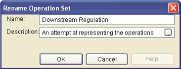
Figure 11.3 Rename Operation Set

11.2.3 Copying an Operation Set

To copy (or duplicate) an operation set:

Select the Operation set you want to copy from the Operation Set list on the Operations tab.
Select Duplicate from the Operations menu of the Reservoir Editor. The Duplicate Operation Set dialog box will open (Figure 11.4).
Give the operation set a new Name and a Description.
Click OK to complete the copy process and to close the dialog box.

The new operation set will have a copy of all the zones that were in the original operation set. Each zone in the new operation set will also list the same rules that were used by the original operation set.

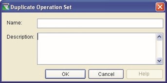
Figure 11.4 Duplicate Operation Set

11.2.4 Deleting an Operation Set

To delete an operation set:

Select Delete from the Operations menu of the Reservoir Editor. The Select Operation Set to Delete dialog box will open (Figure 11.5).

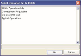
Figure 11.5 Select Operation Set to Delete

Highlight the operation set you wish to delete. Its name should appear in the grey box at the bottom.
Click OK to complete the delete process and to close the dialog box. A confirmation dialog box will appear asking if you really want to delete the selected operation set.

11.2.5 Editing an Operation Set

At the top of the Operations tab, the Operation Set field contains a list of all of the operation sets for your reservoir, with the name of the current operation set displayed. Use this list to select the operation set you wish to edit. The Operations tab will fill with the data for the selected operation set.

Beside the Operation Set name list is the Description of the current operation set; this field is editable. Use the description to describe the purpose of the operation set, the expected behavior the operation set should provide, and any changes you had to make to accomplish your goal. You can enter a much longer description by using the button to access the full text editor for the description.

The remainder of this chapter will detail all the options available for editing your operation set. Each section assumes that you have already created an operation set. If you have not created an operation set, then go back and do so (Section 11.2.1).

11.3 Reservoir Operation Zones

As illustrated in Figure 11.6, when you create a new Operation Set, ResSim automatically creates a Zone-Rules tab that contains three default reservoir operation zones: Flood Control, Conservation, and Inactive. You may wish to rename these default zones and add descriptions. You may need to define additional zones as well. This section will detail how to edit the zone definitions of your operation set.

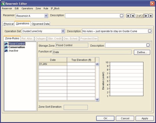
Figure 11.6 Reservoir Editor Showing New Operation Set

11.3.1 Renaming and Describing Operation Zones

To change the name of a Zone as it appears in the operations tree and/or edit its description:

Select the Zone (to be renamed) in the operations tree.
Select Rename from the Zone menu or select Rename from the shortcut menu by right-clicking on the zone you wish to rename in the operations tree. Enter the new name and/or description. The Description field for the Storage Zone is also editable in the Edit panel of the reservoir editor.

Any changes you make to the Storage Zone name will be reflected in the operations tree.

Renaming the Inactive zone does not change its nature. The inactive zone is still a special zone from which the reservoir cannot release water and no rules can be applied to this zone.

11.3.2 Adding a New Reservoir Storage Zone

To add a new Reservoir Storage Zone:

Select New from the Zone menu of the Reservoir Editor. The New Zone dialog box will open (Figure 11.7).
Enter a Name and Description for the new zone.
Click OK to complete the zone creation and close the New Zone dialog box.

Figure 11.7 New Zone

The new zone you created now appears in the operations tree. Complete the process of creating the zone by defining the curve that represents the top of the zone, as explained in the next section.

11.3.3 Defining Operation Zones

You will need to define the curves representing the top of each zone you have created. The default definition of a zone includes a table of dates and elevations. The first date in the table is always 01Jan. The curve is defined by straight lines connecting the points defined in the table, and the last point connects back to the first point as the year repeats.

The top of zone can also be defined using a flexible zone definition. For example, if the top of zone varies from year to year, then it can be defined as a function of an external time series by reading the top of zone from HEC-DSS. Or, if the top of zone is a function of a model variable or a state variable, it can be defined using the Define button.

When the selected feature in the operations tree is a Zone, the Zone Editor is displayed in the Edit Panel and the mini-plot at the right will illustrate the curves representing the top of each zone. The color of the selected zone's curve will be red. All other zones will be black.

Figure 11.8 shows the curve definition for a zone named Conservation.

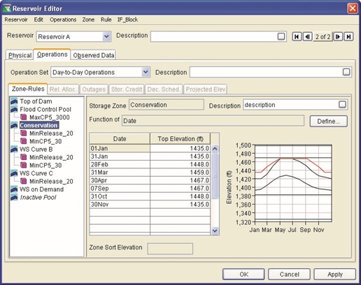
Figure 11.8 Reservoir Editor--Operations Tab: Zone Editor

To define the top of zone curves, do the following for each zone:

Select the Zone in the operations tree to access the Zone Editor containing the data for that zone.
For the default zone definition, enter the Date and Top Elevation values in the table to define the curve for the zone. You can either copy and paste data from a spreadsheet application or type in the values manually. Note that dates often do not copy and paste correctly and must be entered manually.

Be careful when copying "Date" data from a spreadsheet. Most spreadsheet applications use their own specialized numeric format for dates. Only 'text' can be pasted into a date cell in ResSim.

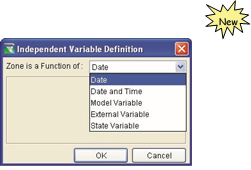Dates are entered in a ddmmm format with the month as a threeletter abbreviation. Dates can also be entered with the calendar tool (which can be accessed by double-clicking in a date cell and then clicking the small ellipse button that appears on the right side of the cell).

Optionally, to use the

flexible zone definition feature, click the "Function of:" Define button, which will open the Independent Variable Definition editor (Figure 11.9). Use this feature when the zone definition is a function of:

Date (default, see step 2 above),

Date and Time, Model Variable, External Variable, or State

Figure 11.9 Independent Variable Definition: "Zone is a Function of:" Selection

Variable. When the zone is not a function of date (or date and time), then a Zone Sort Elevation value will be required to appropriately sort the zones in the ZoneRules tree.

a. Date and Time option (Figure 11.10): enter the appropriate dates and times along with the top of zone elevation values.

Figure 11.10 Flexible Zone Definition – Date and Time

a. Model Variable option (Figure 11.11): from the Independent Variable Definition editor, select the independent variable using the scrollable list and/or using the Filter chooser. If the model variable is not part of the current reservoir for which the zone is being defined, you may need to "un-filter" the Time-Series column. This is accomplished by clicking on the dropdown list, then clicking on the top of the list where you will see a blank line.

At that point, you should see all model variables available for selection.

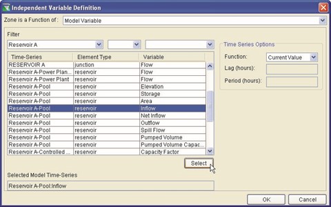
Figure 11.11 Flexible Zone Definition – Model Variable

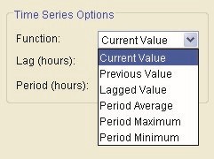Next, you need to define the independent variable with respect to each time step by selecting the appropriate Time Series Options. From the

Function list (Figure

11.12), you can select:

^{Current Value,}Figure 11.12 Time Series Options

Previous Value, Lagged for Flexible Zone Definition Value, Period Average,

Period Maximum, or Period Minimum. The Lag (in hours) can be specified (for all but Current and Previous value) along with the appropriate Period (in hours).

After you have selected the independent variable and defined the appropriate Time Series Options, then you will enter the relationship values between the Independent Variable (in the column labeled with the parameter name of the independent variable, e.g. Flow) and the top of zone elevation value (in the column labeled Top Elevation), as shown in Figure 11.13.

Figure 11.13 Flexible Zone Definition – Model Variable

Relationship Table Definition

b. External Variable option (Figure 11.14): the name of the independent variable is defined using a Variable Name in the form of "Reservoir name-Zone name".

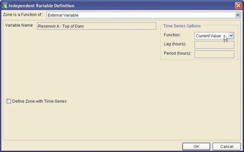
Figure 11.14 Flexible Zone Definition – External Variable

After you have defined the appropriate Time Series Options, then you will enter the relationship values between the External Variable (in the column labeled with the "Reservoir name-Zone name") and the top of zone elevation values in the column labeled Top Elevation (Figure 11.15).

Figure 11.15 Flexible Zone Definition – External Variable

Relationship Table Definition

Alternately, you can click

in the checkbox next to Define Zone with Time-Series. Either of the two external variable choices will cause the "Reservoir name-Zone name" Variable Name to appear on the time-series tab of the Alternative Editor (Chapter 13, Section 13.8).

c. State Variable option (Figure 11.16): select the State Variable from the list. The state variable must be defined prior to creating a flexible zone function that uses it (see documentation of State Variables in Section 11.13.1).

Figure 11.16 Flexible Zone Definition – State Variable

After you have defined the appropriate Time Series Options, then you will enter the relationship values between the State Variable (in the column labeled with the state variable parameter name) and the top of zone

elevation values in the column labeled Top Elevation

(Figure 11.17).

Figure 11.17 Flexible Zone Definition – State Variable

Relationship Table Definition

4. When you have finished entering top of zone curves for a zone, be sure to click the Apply button before moving on to the next zone.

Be careful when defining each zone curve – zones MUST NOT cross each other.

11.3.4 Deleting Operation Zones

To delete a zone from an operation set:

Select the Zone you wish to delete from the operations tree.
Select Delete from the Zone menu or select Delete from the shortcut menu by right-clicking on the zone you wish to delete in the operations tree.
Click OK in the Delete Storage Zone dialog box to complete the delete process.

The Inactive Zone is a special zone in the operation set. If you delete the Inactive Zone from the operation set, it cannot be reestablished.

11.4 Understanding Reservoir Operation Rules

Operation Rules represent the flow goals and constraints upon the releases for each zone of the operation set. Each zone can contain a different set of rules depending on the flow limits and requirements of that zone within the regulation plan. As previously described in Section 11.3.3 and illustrated in Figure 11.8, the rules and zones appear in the Operations Tree on the left side of the Reservoir Editor's Operations tab window.

11.4.1 Release Decision Process

When a set of rules exist within a reservoir zone, the decision logic first determines what the release would be for Guide Curve operation (Section 11.7). Then, working from the "lowest to the highest" priority rule, the program adjusts the release to meet each rule. If two rules contradict each other, the higher priority rule applies (see Section 11.4.5 for a description of prioritizing rules).

The release decision process has 3 basic steps:

Identify the maximum and minimum physical limits on the release. This is the allowable release range.
Narrow the allowable release range by applying the rules in the current zone, starting with the highest priority rule (see Section 11.4.5 for a description of prioritizing rules). For example, if a higher priority rule defines a more restrictive limit on the range than is currently defined by a lower priority rule, then the more restrictive limit is applied. However, if a higher priority rule defines a release limit which allows all the releases in the current release range defined by lower priority rules, then the higher priority rule has no effect on the release range.
Evaluate the desired release for the basic Guide Curve operation (Section 11.7). This is the release needed to get the reservoir to the guide curve in the current time step (computation interval) based on the starting pool elevation, the prior release, and the current inflow.

If the desired release falls within the allowable release range, then the release decision will be the desired release determined in Step 3 above. However, if the desired release is outside the allowable release range determined in the first two steps above, the release will be set to the limit closest to the desired value.

11.4.2 Using Existing Rules

Once you have defined a rule, you can include it in more than one zone by selecting Use Existing from the Rule menu of the Reservoir Editor.

Rules belong to the Reservoir in the current Network, not to a zone or to an operation set. Therefore, any given rule can be used in more than one zone and in more than one operation set. So, be careful – a change to a reservoir's rule in one operation set carries through all operation sets in the current Network that use that rule.

11.4.3 Removing Rules

You can remove a rule from a zone by highlighting the rule in the operations tree and then selecting Remove from the shortcut menu (or select Remove from Zone from the Rule menu of the Reservoir Editor). You can also remove the rule from "all zones" by selecting Remove

Rule From All Zones from the shortcut menu (or select Remove from All Zones from the Rule menu). Similarly, you can remove "all rules" from a zone by highlighting the zone and then select Remove All Rules in this Zone from the shortcut menu (or from the Zone menu, select Remove all Rules). Removing a rule from a zone does not delete the rule. The rule still exists in the reservoir for inclusion in other zones and operation sets.

11.4.4 Deleting Rules

To delete a rule from the reservoir, you can use the Delete option from the Rule menu. Use caution when deleting rules. When you delete a rule, it will no longer be available in any of the zones in this, or any other, operation set for this reservoir in the current reservoir network.

11.4.5 Prioritizing Rules

You must prioritize the rules within a zone, with the highest priority rule being at the top of the list. To raise or lower the priority of a rule within the rule list for the current zone, use the Increase/Decrease Priority or Move to Top/Bottom options in the rule's shortcut menu or from the Rule menu. In Section 11.5, pay special attention to the discussion for each rule type. Some rules, such as the Induced Surcharge rule (Section 11.5.6), may need to be the highest priority rule in a zone.

11.4.6 Renaming Rules

To rename a rule, highlight the rule in the operations tree and select Rename from the shortcut menu (or select Rename from the Rule menu of the Reservoir Editor). Use caution when renaming rules. If you rename a rule, all instances of the rule will be renamed (i.e., the rule's existence within all reservoir zones and operations sets for the reservoir in the current reservoir network).

11.5 Defining Reservoir Operation Rules

This section explains how to define a variety of rules using the different rule types available in ResSim for reservoir Pools, Outlets, and Outlet Groups. Rule types differ depending on whether you apply the rule to the reservoir Pool, a Dam (or Diverted Outlet), an Outlet Group, a Controlled Outlet, a Power Plant, or a Pump. The Operations tab of the Reservoir Editor provides a separate editor for each rule type, as listed below and described in subsequent sub-sections.

Rules for the Reservoir Pool include:

Release Function
Downstream Control Function
Tandem Operation
Induced Surcharge
Flow Rate of Change Limit
Elevation Rate of Change Limit
Script

Rules for the Dam (and for Diverted Outlets and for Outlet Groups and for Controlled Outlets) are as follows:

Release Function
Flow Rate of Change Limit
Script

Rules for Power Plants are as follows:

Release Function
Flow Rate of Change Limit
Hydropower Requirements:
o Hydropower Schedule – Regular o Hydropower Schedule – Time Series o Hydropower Schedule – System o Power Guide Curve
Script

Rule for a Pump is as follows:

Pump Schedule

11.5.1 Adding a New Operation Rule to a Zone

When you create a rule, you must name it, assign the rule to a specific sub-element of the reservoir, and select the rule type. The list of available sub-elements includes: the reservoir Pool (identified by the name of the reservoir); the Dam (identified by the reservoir name hyphenated with the dam name); Diverted Outlets; Outlet Groups, Controlled Outlets; Power Plants; and Pumps.

To add a new operation rule to a zone:

Highlight the appropriate Zone in the operations tree.
Select New from the Rule menu of the Reservoir Editor. The New Operating Rule dialog box will open.
Select the control element of the reservoir to which you will assign this rule (reservoir pool, dam, outlet group, outlet) from the Operates Release from list (Figure 11.18).

Figure 11.18 New Operating Rule

Select the Rule Type from the list. The available rule types will depend upon whether you have selected a pool, dam, outlet, etc., as listed in Section 11.5
Enter a Name for the new rule.
Click OK to close the New Operating Rule dialog box.

The new rule will appear, highlighted, in the operations tree and the edit panel will display the rule editor based on the rule type. The first two fields for each rule editor contain the name of the rule and its description. A description of the rule can be added or changed whenever the rule editor is displayed in the edit panel. See the following sections to determine how to define the appropriate data for your new rule.

11.5.2 Adding an Existing Rule to a Zone

Once you have created a rule in a zone, you may want to use that same rule in another zone.

To add an existing operation rule to a zone:

Highlight the appropriate Zone in the operations tree.
Select Use Existing from the Rule menu of the Reservoir Editor or
Use Existing Rule from the zone's shortcut menu. The Select Existing Rule dialog box will open (similar to Figure 11.19 which shows an example list of existing rules).

Figure 11.19 Select Existing Rule

Select the rule you want to add from the list. Only those rules defined for the current reservoir but not yet used in the current zone will be available for selection. Rules that are being used in the current zone are included in the list, but they are grayed-out. If you want to add the selected rule to all of the zones, then you can check the box labeled Add Rule To All Zones.
Click OK to complete the Use Existing process and close the dialog box.

11.5.3 Defining a Release Function Rule

The Release Function rule type is one of the two most powerful rule types available (the other being the Downstream Control Function rule). With this rule type, you can define a wide array of "function of" rules, meaning release is a function of date or pool elevation, etc. This rule can be assigned to any of the release elements (pool, dam, or outlet) and it allows you to specify the maximum, minimum, or specified flow to be released through the release element.

Use specified limit type rules with caution. Most operation rules describe either a minimum or maximum limit. Specified rules describe the precise amount of flow to be released, neither more or less, making them effectively both a minimum and a maximum limit at the same time. Therefore, a specified release rule is very restrictive because it sets the allowable range of the release to a single value.

The simplest rules defined with this rule type are those where the release limit is a function of date. Rules of this type are seasonally-varying release limits. For example: "the maximum release from the reservoir during the growing season is 6500 cfs and 8500 cfs during the nongrowing season".

The more complex rules that can be created with the Release Function rule type are those where the release limit is a function of an internal (model) variable or an external variable or a state variable. For example, a complex rule might be where the minimum release is a function of the inflow to the reservoir. Inflow to the reservoir is just one of many internal or "model" variables that can be used to create a "function of model variable" rule. The "function of external variable" rule is also very powerful, limited only by your imagination and the time-series data available. An example of an "external variable" rule might be one where the minimum release is a function of dissolved oxygen at a specific gage. Since ResSim cannot compute dissolved oxygen, a timeseries record that describes the predicted or observed values for that variable would be used to influence the release based on the function you define. Using a "state variable" within a release function rule opens up an endless possibility of options available for describing the operation of a reservoir.

To define a Release Function rule:

To create a new Release Function rule, follow the instructions in Section 11.5.1. Be sure to select Release Function for the Rule Type in the New Operating Rule editor.
Highlight the appropriate rule in the operations tree to access the Release Function rule editor (Figure 11.20). The name and description of the rule will appear in the Rule Name and Description fields.

Figure 11.20 Reservoir Editor--Operations Tab:

New Release Function Rule

Define the Limit Type by selecting Minimum, Maximum, or Specified from the dropdown list.
Define the Release Function. Click the "Function of:" Define… button. The Independent Variable Definition editor will open (Figure 11.21).

Figure 11.21 Release Function Rule, Selecting a

Function from Independent Variable Definition Editor

Select the function type from the "Release is a Function of" list: Date, Date and Time, Model Variable, External Variable, or State Variable.

If the function type is Model Variable, select the independent variable using the Filter chooser (Figure 11.22).

Figure 11.22 Release Function Rule, Select an

Independent Variable from the

Model Variable List

If the function type is External Variable, identify the independent variable in the name field (Figure 11.23). This name will appear on the time-series tab of the Alternative Editor (Chapter 13, Section 13.8).

Figure 11.23 Release Function Rule, Defining an

External Variable as the

Independent Variable

If the function type is State Variable, select the State Variable from the list (Figure 11.24). The state variable must be defined prior to creating a release function rule that uses it (see documentation of State Variables in Section 11.13.1).

Figure 11.24 Release Function Rule, Select a State Variable as the Independent Variable

If desired, for either the Model

Variable, or the External Variable, or the State Variable, select from their editors the

Time Series Options (Figure 11.25) to define the

independent variable with

respect to each time step. From the Function list, you can Figure 11.25 Time Series select: Current Value, Options for Model, External,

Previous Value, Lagged and State Variables

Value, Period Average, Period Maximum, or Period Minimum. The Lag (in hours) can be specified (for all but Current and Previous value) along with the appropriate Period (in hours).

Click OK to complete the definition of the independent variable of your function.
Verify that the Limit Type is defined appropriately (as Minimum, Maximum or Specified).

Select the Interpolation Type as Linear, Cubic, or Step (see Section
11.6.1 for a description of how the interpolation types work).
Define the function using the table in the release function rule editor (Figure 11.26). You can either copy and paste data from a spreadsheet application or type in the values manually.

Be careful when copying date data from a spreadsheet. Most spreadsheet applications use their own specialized numeric format for dates. Only 'text' can be pasted into a date cell in ResSim.

The mini-plot will reflect the values you enter and can be viewed in full size when you double-click on it.

If using a function of date, you can enter a single value for 01 Jan to describe a constant release limit throughout the year or enter multiple dates to define a seasonally varying release limit rule. Dates can also be entered with the calendar tool, which can be accessed by double-clicking in a date cell then clicking the ellipse button that appears. As a date entry option, use the calendar tool to set day and month for the date; although the year appears in the calendar tool, it is ignored in setting the date.
If your rule is a function of a variable, you can make your rule seasonally varying by using the Seasonal Variation option. Refer to Section 11.6.6 for more details.
If you wish to use Hour of Day or Day of the Week Multipliers, refer to Sections 11.6.3 and 11.6.4 for more details.
To make your rule applicable only under rising (or falling) conditions, use the Rising/Falling Condition option. Refer to Section 11.6.5 for details.

Check the position of your new rule with respect to the other rules in this zone. To raise or lower the priority of a rule within the rule list for the current zone, use the Increase/Decrease Priority or Move to Top/Bottom options in the rule's shortcut menu or from the Rule menu.

An example of a completed Release Function rule is shown in Figure 11.26. When you have finished entering data for the Release Function rule, be sure to click the Apply button before moving on to the next rule. When copying and pasting cells from a spreadsheet to the table, only the top left cell needs to be selected before pasting. The table will automatically populate with the required rows.

Figure 11.26 Example of Completed Release Function Rule

11.5.4 Defining a Downstream Control Function Rule

This rule type (and its editor) is an extension of the Release Function rule described in Section 11.5.3. Downstream control rules describe the minimum or maximum flow (e.g., flow requirement or channel capacity) or stage at a control point rather than an explicit limit on the release. The final release limit will be determined based on the influence of routing and cumulative local flows at the downstream control point, including the use of an optional contingency applied to the cumulative local flows.

In addition, the Downstream Control rules can be used to create system operation (where two or more parallel reservoirs are operated to have balanced storages while controlling for common downstream requirements). Once created for one reservoir, the Downstream Control rule will also be available in the List of Existing Rules (refer to Section 11.5.2) for other reservoirs in the network. To establish a system operation, the same downstream control rule must be used in each applicable reservoir's operation set. Chapter 12 discusses ResSim's methodology for system operation and storage balancing.

The Downstream Control rule can be assigned only to the reservoir (pool), not to a specific outlet or outlet group, because only the reservoir can account for all releases from the reservoir's outlets that could influence the flow at the downstream control point.

Entering operations data for a Downstream Control Function rule:

To create a downstream control rule, follow the instructions for creating a new rule as described in Section 11.5.1. After selecting the Operate Release From to be the reservoir and the Rule Type to be Downstream Control Function, be sure to select the downstream control point from the Downstream Location list that appears when you select the Downstream Control Function rule type. Figure 11.27 illustrates the creation of a Downstream Control Function rule.

Figure 11.27 Reservoir Editor--New Operating Rule: Downstream Control Function

The Downstream Control Function rule editor (Figure 11.28) is essentially the same as the Release Function rule editor. However, there are three significant differences that you have the option of using:
- Define the rule as a minimum or maximum Flow or Stage
parameter limit at the downstream control point (see in a Figure 11.28)
- Specify a Flow Contingency for the cumulative local flows at the downstream control point (see in Figure 11.28) b
- Specify Advanced Options that relate to how routing attenuation and rate of change constraints are considered during the operation for downstream rules in general (global values) or for a specific downstream rule (see in Figure 11.28) c

Figure 11.28 Reservoir Editor--Example of a Downstream

Control Function Rule

The three options specific to the Downstream Control rule (as shown in Figure 11.28) are described as follows:

Select the appropriate Parameter (Flow or Stage) that should be used for the downstream operation. The column heading in the table will reflect the chosen parameter.

Figure 11.29 Flow Contingency for Downstream

Operation

If a constant contingency is desired, then click on the radio button for the Constant Contingency percentage % and enter a percentage value. For example, a value of 20 would indicate that during the release decision process, the cumulative local flows would be increased by 20%, thus reducing the amount of space available at the downstream location. A negative contingency value (e.g., -20) decreases the cumulative local flows, thus increasing the amount of space available at the downstream location.
If variable contingency values are desired, then click on the radio button for the Contingency percentage as a function of Cumulative local flow and enter the table of cumulative local flow values vs. percent contingency values. As with the constant contingency described above, the space available at the downstream location is influenced by the sign and magnitude of the contingency values.

To specify how routing attenuation and rate of change constraints will be handled during the downstream operation logic:

Click the Advanced Options button and the Advanced Options editor will open (left portion in Figure 11.30) where you will see the radio button selected to Use Global Options.
To change the Global options (which applies to all downstream rules at all reservoirs), click on the Edit button, which will open the Global Downstream Options editor (right portion in Figure 11.30.

Figure 11.30 Advanced Options for Downstream Rule(s) – Global Options

To change the Rule Specific options (which applies only to the downstream rule being edited), click on the radio button Use Rule Specific Options. The lower portion of the Advanced Options editor will become available for editing (Figure 11.31)

Figure 11.31 Advanced Options for

Downstream Rule – Rule Specific Options

The same advanced options are available for both the global options and the rule specific options. These options are divided into two subject areas: routing attenuation and rate of change.

Correct for Attenuation: Depending on the routing method and parameters being used for the routing reaches between the operating reservoir and the downstream location, this option will allow for adjustments to be made in the release decision process with consideration of the routing attenuation parameter (i.e., the routed hydrograph "shaping" parameter).
- Option 1 (Lagged Space Adjustment) – enter Max Iterations, an Absolute Flow Tolerance (cfs or cms), and a Tolerance Fraction of Limit (%).
- Option 2 (Predictor Corrector) – enter Max

Iterations and a Correction Factor (from zero to one).

No Correction – select this option when you do not want any adjustments made based on the routing attenuation parameters.

 Rate of Change Constraints: When the reservoir operations include rate of change constraints, there may be a conflict between operating for downstream constraints (i.e., wanting to cut back releases to reduce downstream flooding) vs. rate of change constraints (i.e., not able to cut back fast enough). This option allows the modeler to Consider ROC Constraints and specify a Max Lookahead for ROC (Number of Time Steps).

The Reset Parameters button will make the

options return to their original values.

Note: Since these Advanced Options are complex, "trial and error" runs might be needed to test their impact on downstream operations.

Check the position of your new rule with respect to other rules in the zone it is placed. To raise or lower the priority of a rule within the rule list for a particular zone, use the Increase/Decrease Priority or Move to Top/Bottom options in the rule's shortcut menu or from the Rule menu.
When you have finished entering data for the Downstream Control Function rule, be sure to click the Apply button before moving on to the next rule.

As a visual reference, after a downstream control rule has been defined, the downstream location in the display area (i.e., the watershed map) will have a box drawn around the junction symbol.

11.5.5 Defining a Tandem Operation Rule

A Tandem Operation rule establishes a tandem system operation where an upstream reservoir operates for a downstream reservoir to achieve a storage balance. Unlike the Downstream Control rule (which is the only other rule type used for system operation and must be included in the operation sets of all reservoirs in the system), the Tandem Operation rule is created and included in the operation set at the upstream reservoir only. The Tandem Operation rule simply identifies the downstream reservoir that is the object of tandem operation. An implicit (default) storage balance scheme is invoked by the Tandem Operation rule, and an optional explicit (user-defined) storage balance scheme can be defined and used instead of the default (refer to Chapter 12 for more discussion on system operation).

When creating the Tandem Operation rule, it can be assigned only to the reservoir (pool), not to a specific outlet or outlet group, because only the reservoir can account for all releases from the reservoir's outlets that could influence the flow into the downstream reservoir.

To enter operations data for a Tandem Operation rule:

To create a Tandem Operation rule, follow the instructions for creating a new rule as described in Section 11.5.1. Be sure to select the reservoir for the release component (Operates Release from) and Tandem Operation for the Rule Type in the New Operating Rule editor. Figure 11.32 illustrates the creation of a Tandem Operation rule.

Figure 11.32 Reservoir Editor--New Operating Rule:

Tandem Operation

To define your Tandem Operation rule, highlight the rule in the operations tree of the reservoir editor (Figure 11.33). In the Edit Panel, you can enter a Description, and most importantly select the Downstream Reservoir for which the current (upstream) reservoir is operating.

Figure 11.33 Reservoir Editor--Example of a

Tandem Operation Rule

Check the position of your new rule with respect to other rules in the zone it is placed. To raise or lower the priority of a rule within the rule list for a particular zone, use the Increase/Decrease Priority or Move to Top/Bottom options in the rule's shortcut menu or from the Rule menu.
When you have finished setting up the Tandem Operation rule, be sure to click the Apply button before moving on to the next rule.

11.5.6 Defining an Induced Surcharge Rule

Induced Surcharge is a flood control operation that specifies emergency releases when the current pool elevation and rate of increase in inflow (or change in pool elevation) threaten to overtop the dam. This operation may necessitate releases that exceed channel capacity constraints. A reservoir must have a gated outlet to employ induced surcharge operations.

Induced Surcharge operation is achieved by physically regulating the position of spillway gates. When the gate opening is reduced to limit release to less than free overflow (the fully-open position), water is intentionally surcharged—or stored—behind the gates. For this reason, induced surcharge is also referred to as a gate regulation operation. Induced Surcharge operation allows operators to better manage a flood event by using additional reservoir storage volume above the spillway crest.

In HEC-ResSim, the Induced Surcharge rule must be defined and entered as the highest priority rule in every zone spanning elevations between the top of the dam and the lowest elevation from which the gate can be regulated, generally, the controlled spillway crest. Additionally, a Release Function rule (Section 11.5.3) with Limit Type set to Maximum must be defined and entered as a lower priority rule in each of the applicable zones (below the induced surcharge rule). This maximum flow corresponds to the maximum discharge when surcharge operations are not in effect. It is essential to enter this maximum flow limit to guide releases back towards flood control operations after surcharge operations finish. Note that when creating a new rule, the Induced Surcharge option is only available if the "reservoir itself" is selected for Operates Release from: ("Sayers" in Figure 11.34, not "Sayers-Dam" or "Sayers-Gate").

Figure 11.34 Reservoir Editor--Operations Tab:

Create Induced Surcharge Rule

Within the Induced Surcharge rule editor, there are two options for defining the rule:

Use Induced Surcharge Function (Section 11.5.6.1)
Specify the ESRD Curves (Section 11.5.6.2)

11.5.6.1 Induced Surcharge Function Option

If you select the option (as shown in

Figure 11.35 for Sayers reservoir), then the Induced Surcharge Envelope Curve, Time of Recession, and Falling Pool Options determine the magnitude and duration of gate-regulated releases, and how emergency release should transition back to normal flood control releases.

Figure 11.35 Induced Surcharge Rule Editor,

Use Induced Surcharge Function Option

To enter operational data for an Induced Surcharge rule using the Induced Surcharge Function:

Highlight the induced surcharge rule in the operations tree to access the Induced Surcharge rule editor. The name and description of the rule will appear in the Induced Surcharge Rule and Description fields.
Select the radio button for Use Induced Surcharge Function.
Select the Interpolation Type as Linear or Cubic (Section 11.6.1).
Enter Elevation and Release data into the table to describe the Induced Surcharge Envelope. This envelope defines the lower limit of allowable regulated release when the pool is at a certain elevation. The rule will compute a higher release as described in EM 1110-2-
3600 (USACE, 1987). You can either copy and paste data from a spreadsheet application or type in the values manually.
Enter the Time of Recession in hours. This constant describes the length of time an incoming flood is expected to take to recede. The program uses this time to compute the volume of water that must be evacuated to prevent overtopping the dam. See discussion in EM 1110-2-3600 (USACE, 1987) for further documentation regarding the Recession Time constant parameter (Ts).
At this point, the Induced Surcharge rule editor should appear similar to the Sayers reservoir example (Figure 11.36) illustrating the use of the Induced Surcharge Function.

Figure 11.36 Induced Surcharge Rule Editor,

Completed Example of Induced Surcharge Function

To see a plot containing the computed Induced Surcharge Curves (Figure 11.37) based on the data you have entered, double-click on the mini-plot located to the right of the table (or, you can right-click on the mini-plot and select Show popup).

Figure 11.37 Plot of Computed Induced Surcharge Curves

(with the Discharge Capacity Curve)

The Induced Surcharge Curves Plot menu bar consists of the

"generic" File, Edit, and View menus that are described in Chapter

14 (Section 14.5.2) and in Appendix F.

The Options menu (Figure 11.38) is specific to the Induced Surcharge Curve Plot and contains the following options to allow access to the Inflow and Rate of Rise editors:

Edit Inflows for Curves… Allows for specifying the inflow values which may be used in displaying an example plot of induced surcharge release curves in the zone below the envelope curve. Figure 11.39 shows the inflow values corresponding to the inflow curves.
Plot Rate Of Rise will generate a plot of the rate of rise curves (if given). When this option is checked, the "Edit Rate of Rise for Curves …" option appears in place of the "Edit Inflows for Curves…" option.

Figure 11.38 Options

Menu (from Induced

Surcharge Curves Plot)

Figure 11.39 Edit Inflow for Curves… (from Options Menu of Induced Surcharge Curves Plot)

Show Discharge Capacity is a toggle to indicate whether or not to include the Discharge Capacity Curve in the plot. Figure 11.40 shows the Induced Surcharge Curves Plot without the Discharge Capacity Curve.

Figure 11.40 Plot of Computed Induced Surcharge Curves

(without the Discharge Capacity Curve)

Section 11.5.6.3 describes the Falling Pool Options and the Inflow Time Series Options.
Check the position of your new rule with respect to the other rules in this zone. To raise or lower the priority of a rule within the rule list for the current zone, use the Increase/Decrease Priority or Move to Top/Bottom options in the rule's shortcut menu or from the Rule menu.
When you have finished entering data for the Induced Surcharge rule, be sure to click the Apply button before moving on to the next rule.

11.5.6.2 Specify the ESRD Curves Option

If you select the option (Figure 11.41) to

specify the Emergency Spillway Release Diagram (ESRD) curves, then the Elevation vs. Min Release per Inflow (or Elevation vs. Min Release per Rate of Rise) relationship is used along with the Falling Pool Options to determine the magnitude and duration of gate-regulated releases, and how emergency release should transition back to normal flood control releases.

Figure 11.41 Induced Surcharge Rule Editor,

Specify the ESRD Curves Option

To enter operational data for an Induced Surcharge rule specifying the ESRD Curves:

Highlight the induced surcharge rule in the operations tree to access the Induced Surcharge rule editor. The name and description of the rule will appear in the Induced Surcharge Rule and Description fields.
Select the radio button for Specify the ESRD Curves.
Specify Releases with Respect to: either Reservoir Inflow or Rate of Rise
Select the Edit Inflows for ESRD Curves… button and the dialog box will open (Figure 11.42) where you will enter the appropriate values (either Reservoir Inflows or Rate of Rise) for the subsequent definition of the ESRD curves.

Figure 11.42 Induced Surcharge Rule – Entering

ESRD Values (Inflows or Rate of Rise)

Enter Elevation and Min Release data into the Elevation vs. Min Release per Inflow table to describe the family of curves. These release values define the lower limit of allowable regulated release when the pool is at a certain elevation and the inflow is a certain amount. You can either copy and paste data from a spreadsheet application or type in the values manually.
At this point, the Induced Surcharge rule editor should appear similar to the example in Figure 11.43 illustrating the use of the ESRD Curves.

Figure 11.43 Induced Surcharge Rule Editor,

Completed Example of Specifying the ESRD Curves

To see a plot containing the family of ESRD Curves (Figure 11.44) based on the data you have entered, double-click on the mini-plot located to the right of the table (or, you can right-click on the miniplot and select Show popup).

Figure 11.44 Plot of Induced Surcharge Curves for Specified ESRD Inflow Values

The Induced Surcharge Curves Plot menu bar consists of the "generic" File, Edit, and View menus that are described in Chapter 14 (Section 14.5.2) and in Appendix F.

Section 11.5.6.3 describes the Falling Pool Options and the Inflow Time Series Options.
Check the position of your new rule with respect to the other rules in this zone. To raise or lower the priority of a rule within the rule list for the current zone, use the Increase/Decrease Priority or Move to Top/Bottom options in the rule's shortcut menu or from the Rule menu.
When you have finished entering data for the Induced Surcharge rule, be sure to click the Apply button before moving on to the next rule.

11.5.6.3 Falling Pool and Inflow Time Series Options

There are two options that apply to either one of the Induced Surcharge rule definition options (Use Induced Surcharge Function or Specify the ESRD Curves). These two options are:

Falling Pool
Inflow Time Series

a. Select Falling Pool Options by

clicking the Edit button beside the Falling Pool Options label. The Falling Pool Options dialog box will open (Figure 11.45).

Figure 11.45 Induced Surcharge -- Falling Pool Options

Enter the Time for Pool Decrease in hours. This parameter describes the required number of successive hours the reservoir pool level must be falling before transitioning from rising pool emergency spillway releases to falling pool releases.
Enter the Falling Pool Transition Elevation in feet (meters).
This parameter represents the pool elevation above which Falling Pool releases will be made. Once the pool elevation falls below this elevation, the Induced Surcharge rule will no longer operate, and ResSim will resume releases based on other rules in the active zone.
For Release Options, choose Ratio of Inflow, Average of Inflow and Previous Release, Maintain Peak Release, or Maintain Peak Gate Openings to designate the method for computing falling pool releases. Falling Pool Releases will be made after the pool begins to fall and until the pool level returns to the Falling Pool Transition Elevation.
- For Ratio of Inflow, enter the Release ratio times inflow averaged over number of hours.
- For Avg of Inflow and Previous Release, enter the number of hours for the Inflow to be averaged over.
- Maintain Peak Release indicates that the maximum release will be held until surcharge operation is no longer applicable and normal operations are resumed.
- Maintain Peak Gate Openings indicates that the maximum gate opening will be maintained until surcharge operation is no longer applicable and normal operations are resumed.
 Click OK to close the Falling Pool Options dialog and a checkmark will display in the box beside Falling Pool Options in the Reservoir Editor.

b. Pressing the Inflow Time Series

Options button activates the Inflow Time Series Options editor (Figure 11.46). This editor defines how the reservoir inflow time series is interpreted when used in making induced surcharge operation release decisions.

Figure 11.46 Induced Surcharge --

Inflow Time Series Options

The Function list includes Current Value, Previous Value, Lagged Value, Period Average, Period Maximum and Period Minimum.
Enter the optional Lag (in hours) for all functions except Current and Previous.
The Period (in hours) is applicable for Period Average, Period Maximum and Period Minimum functions.

11.5.7 Defining a Flow Rate of Change Limit Rule

A Flow Rate of Change Limit rule specifies the allowable change when increasing or decreasing release values (i.e., "ramping rates"). A single rule of this type will only limit a rising release or a falling release, but not both. To describe both increasing and decreasing limits, you must define two rules and set the type of one to increasing and the other to decreasing. A rule of this type can be assigned to any release element to influence the behavior of that element.

To enter operations data for a Flow Rate of Change Limit rule:

To create a new rule, follow the instructions in Section 11.5.1. Be sure to select Flow Rate of Change Limit for the Rule Type in the New Operating Rule editor.
Highlight the appropriate rule in the operations tree to access the Flow Rate of Change Limit rule editor (Figure 11.47). The name and description of the rule will appear in the Release Rate of Change Limit rule and Description fields.

Figure 11.47 Reservoir Editor--Operations Tab: Flow Rate of Change Limit Rule

For Function Of:, select either Constant, Reservoir Inflow, Release, or Pool Elevation.
For Type, select either Increasing or Decreasing.
Enter the Max Rate of Change value. The limit is described in units of flow (cms or cfs) per hour, regardless of the compute interval. For example, if you enter 500 cfs/hr with a compute interval of 12 hours, then this rule describes the maximum flow change per time step as 6000 cfs.
If your Function Of: selection is Constant, enter a single value for the limit.
If your Function Of: selection is Reservoir Inflow, Release, or Pool Elevation, then a table will appear to allow you to describe how the rate of change is influenced by the selected independent variable. Additionally, select the type of Interpolation to apply to the curve as either Linear, Cubic, or Step (Section 11.6.1).
Check the position of your new rule with respect to the other rules in this zone. To raise or lower the priority of a rule within the rule list for the current zone, use the Increase/Decrease Priority or Move to Top/Bottom options in the rule's shortcut menu or from the Rule menu.
When you have finished entering data for the Flow Rate of Change rule, be sure to click the Apply button before moving on to the next rule.

11.5.8 Defining an Elevation Rate of Change Limit Rule

An Elevation Rate of Change Limit rule describes the allowable change when increasing or decreasing pool elevation values. A single rule of this type will only limit a rising pool or a falling pool, but not both. To describe both increasing and decreasing limits, you must define two rules and set the type of one to increasing and the other to decreasing. Since this rule watches the pool elevation, you can assign this rule only to the pool (reservoir), not to the dam or to a discrete outlet.

To enter operations data for an Elevation Rate of Change Limit rule:

To create a new rule, follow the instructions in Section 11.5.1. Be sure to select the reservoir for the Release Element and Elev Rate of Change Limit for the Rule Type in the New Operating Rule editor.
Highlight the appropriate rule in the operations tree to access the Elevation Rate of Change Limit rule editor (Figure 11.48). The name and description of the rule will appear in the Elevation Rate of Change Limit Rule and Description fields.

Figure 11.48 Reservoir Editor--Operations Tab:

Elevation Rate of Change Limit Rule (Pool)

For Function Of:, select either Constant, Reservoir Inflow, or Release.
For Type, select either Increasing or Decreasing.
Choose either Instantaneous or Period Average.

For Instantaneous, enter the Max Rate of Change value in units of meters (feet) per hour.
For Period Average, specify the Max Change and the number of Hours over which the change is allowed.

Check the position of your new rule with respect to the other rules in this zone. To raise or lower the priority of a rule within the rule list for the current zone, use the Increase/Decrease Priority or Move to Top/Bottom options in the rule's shortcut menu or from the Rule menu.
When you have finished entering data for the Elevation Rate of Change Limit rule, be sure to click the Apply button before moving on to the next rule.

11.5.9 Defining Hydropower Rules

Hydropower rules specify the minimum releases needed from a reservoir's power plant (or from the power plants in a reservoir system) to meet a power generation requirement and schedule. The desired release is a function of the plant's generation capacity, the hydraulic head, and the required energy. In the various hydropower rules, the generation requirement can be specified as a function of storage, season, or be directly specified as an external time series.

There are four different Hydropower rule types (Figure 11.49) available for you to create a rule that describes a Hydropower Requirement: Schedule, Time Series, Power Guide Curve and System Schedule. Data entry for these rules will be described in the following subsections.

Figure 11.49 Hydropower Rule Types

11.5.9.1 Hydropower – Schedule

The Hydropower – Schedule rule allows you to define a regular monthly or user specified seasonally varying hydropower requirements. The various options on this rule editor allow you to define each month's power generation requirement, the type of the requirement (megawatt-hours or plant factor), and the hours of the day and days of the week during which the plant can generate.

To define a Hydropower – Schedule Requirement rule:

To create a new rule, follow the instructions in Section 11.5.1. Be sure to select the power plant for the Release Element and then select Hydropower – Schedule for the Rule Type in the New Operating Rule editor.
Highlight the appropriate rule in the operations tree to access the Hydropower – Schedule rule editor (Figure 11.50). The name and description of the rule will appear in the Hydropower – Schedule rule and Description fields.

Figure 11.50 Hydropower – Schedule Rule Editor

Click the Options button to open the Power Generation Requirement editor (Figure 11.51).

From the Requirement
Varies list select either Monthly or Seasonally.
From the Requirement
Specified as list you can select Plant Factor,
Daily Total MWH,
Weekly Total MWH, or Monthly Total MWH.

Figure 11.51 Power Generation

Requirement Options

If Weekly Total MWH is selected from the Requirement Specified as list, then you must select the Starting Day of the power week as one of the seven days of the calendar week. You will also need to select a day of the week, which by its inclusion in both a power week and a month, determines which month to include that power week.

 Finally, select the Period over which the requirement will be satisfied as being Each Time-Step, Daily, or Weekly. If Weekly is selected, then you will need to select the Starting Day of Period.

Complete the power requirement table as appropriate, depending on the options selected in the previous step. For example, if Monthly Requirement in MWH was selected, then enter the total monthly requirement for each month of the year.
Click the Power Generation Pattern button to open the Power Generation Pattern editor. Please see Section 11.5.9.5 for a full description of the purpose and use of the Power Generation Pattern editor.
Check the position of your new rule with respect to the other rules in the zone. To raise or lower the priority of your rule within the rule list for the current zone, use the Increase/Decrease Priority or Move to Top/Bottom options in the rule's shortcut menu or from the Rule menu.
When you have finished entering data for the Hydropower - Schedule rule, be sure to click the Apply button before moving on to the next rule.

11.5.9.2 Hydropower – Time Series Requirement

The Hydropower – Time Series Requirement rule allows you to define an irregular schedule of Hydropower requirements through the use of a DSS time-series record. There are no options in this rule editor. Instead, a message is placed there to remind you that you will need to specify a time series of required power in units of megawatts when you develop an alternative that uses this operation set for this reservoir.

To define a Hydropower – Time Series Requirement rule:

To create a new rule, follow the instructions in Section 11.5.1. Be sure to select the power plant for the Release Element and then select Hydropower – Time Series Requirement for the Rule Type in the New Operating Rule editor.
Highlight the appropriate rule in the operations tree to access the
Hydropower – Time Series Requirement rule editor (Figure
11.52). The name and description of the rule will appear in the Hydropower – Time Series Requirement rule and Description fields.

Figure 11.52 Hydropower – Time Series

Requirement Rule Editor

Make note of the message and the name of the Rule you just created. When you develop an alternative for this network, reservoir, and operation set, you will need to provide a DSS time-series pathname specification for this rule. The entry in the Time Series table of the rule editor will be identified by the rule name with a parameter of power.

11.5.9.3 Hydropower – Power Guide Curve

The Hydropower – Power Guide Curve rule allows you to define a function that describes the hydropower generation requirement with respect to the available storage in the power pool. The power requirement must be described in units of % plant factor.

To define a Hydropower – Power Guide Curve rule:

To create a new rule, follow the instructions in Section 11.5.1. Be sure to select the power plant for the Release Element and then select Hydropower – Power Guide Curve for the Rule Type in the New Operating Rule editor.
Highlight the appropriate rule in the operations tree to access the Hydropower – Power Guide Curve rule editor (Figure 11.53). The name and description of the rule will appear in the Hydropower – Power Guide Curve rule and Description fields.

Figure 11.53 Hydropower – Power Guide Curve Rule Editor

From the lists for Zone at Top of Power Pool and Zone at Bottom of Power Pool, select the top of zone curves that bound the top and bottom of the Power Pool.
Complete the table to define the Power Guide Curve. The first column is the percent of power storage available in the power pool. These values should increase as you move down in the table. The second column is the percent plant factor. This is the power requirement as a percentage of the plant's capacity to generate.
If desired, click the Power Generation Pattern button to open the Power Generation Pattern editor. Please see Section 11.5.9.5 for a full description of the purpose and use of the Power Generation Pattern editor.
Check the position of your new rule with respect to the other rules in the zone. To raise or lower the priority of your rule within the rule list for the current zone, use the Increase/Decrease Priority or Move to Top/Bottom options in the rule's shortcut menu or from the Rule menu.
When you have finished entering data for the Hydropower – Power Guide Curve rule, be sure to click the Apply button before moving on to the next rule.

11.5.9.4 Hydropower – System Schedule

The Hydropower – System Schedule rule allows you to specify a hydropower generation requirement that a set of reservoirs (a reservoir system) will operate to try to meet. This rule describes the hydropower generation requirement in the same manner as the at-site hydropower schedule rule (as previously discussed in Section 11.5.9.1) with some additional options for specifying the power generation pattern and for identifying reservoirs whose power generation can be used to meet the system requirement.

Typically, to cause a reservoir to operate to meet a system power requirement, it must have a Hydropower-System Schedule rule in the currently active zone of its operation set. The easiest way to do this is to create the rule in one of the reservoirs. Then, add it to the operation set(s) of the other operating reservoirs in the system by selecting it from the "Use Existing" list.

To define a Hydropower – System Schedule rule:

To create a new rule, follow the instructions in Section 11.5.1. Be sure to select the power plant for the Release Element and then select Hydropower – System Schedule for the Rule Type in the New Operating Rule editor.
Highlight the appropriate rule in the operations tree to access the Hydropower – System Schedule rule editor (Figure 11.54). The name and description of the rule will appear in the Hydropower – System Schedule rule and Description fields.

Figure 11.54 Hydropower – System Schedule Rule Editor

Click the Options button to
open the Power Generation Requirement editor (refer to previous discussion in Section 11.5.9.1, step 3).
Complete the power requirement table as appropriate, depending on the options selected in the previous step. For example, if Monthly Requirement in MWH was selected, then enter the total monthly requirement for each month of the year.
Click the Contributing Reservoirs… button
to open the Hydropower-System Rule: Reservoir List editor (Figure 11.55). Use this editor to select those power-producing reservoirs in your network that do not actively operate for this system hydropower requirement but whose generation can be counted toward meeting it. You need not add reservoirs which will actively operate for this requirement (share this rule), they will be added to the "Selected" list automatically when you add this rule to their operation set(s).

Figure 11.55 Hydropower System Rule:

Reservoir List Editor

There are two choices for indicating the Power Generation Pattern:
- Specify Local Generation Pattern – this option allows you to specify a different generation pattern for each reservoir that operates to meet the system power requirement. If you choose this option, you will need to edit the power pattern in the system hydropower rule from each reservoir that includes the rule in its operation set.
- Specify System Generation Pattern – this option allows you to specify a single generation pattern that will be used by all the reservoirs that operate to meet the system power requirement.
Click the Edit Pattern button to open the
Generation Pattern editor, where you will specify a (local or system) pattern for meeting the system hydropower requirements. Please see Section 11.5.9.5 for a full description of the purpose and use of the Power Generation Pattern editor.
When both a local power rule and a system power rule are specified at a reservoir, the two rules do not "know" about each other's requirement or generation pattern. The two rules will independently develop release requirements for the reservoir which will then be negotiated in the rule stack based on their priority, like any other rule. Note, two power rules applied to a single power plant will not be additive.
Check the position of your new rule with respect to the other rules in the zone. To raise or lower the priority of your rule within the rule list for the current zone, use the Increase/Decrease Priority or Move to Top/Bottom options in the rule's shortcut menu or from the Rule menu.
When you have finished entering data for the Hydropower – System Schedule rule, be sure to click the Apply button before moving on to the next rule.

11.5.9.5 Power Generation Pattern

The Power Generation Pattern allows you to specify a weekly distribution of the specified energy requirements based on the time of the day and day of the week. The pattern covers a week and each day is described with a set of 24 hourly weighting factors. By default, the weekly pattern repeats throughout the year unless you specify a set of seasons and a different pattern for each season.

The Weekly Pattern

Three options are available for specifying the weekly power pattern: All Week, Weekdays and Weekend, and Each Day. These options are available from the Specify Pattern for list.

The All Week option (Figure 11.56) simply applies the same power generation pattern for every day of the week.
The Weekdays and Weekend option (Figure 11.57) allows you to specify a different power generation pattern for Weekdays (Monday through Friday) than for Weekend days (Saturday and Sunday).

Figure 11.56 Power Generation Figure 11.57 Power Generation

Pattern (All Week) Pattern (Weekdays &

Weekends)

The Each Day option (Figure 11.58) allows you to specify different power generation patterns for every day of the week.

Figure 11.58 Power Generation Pattern (Each Day)

Hourly Distribution

Each day of the Power Generation Pattern table is divided into 24 hourly values. Each value represents a weighting factor that you can use to distribute the energy requirement throughout the day and throughout the week. The default value for each hour of the day is 1.0 (Figure 11.59) which will evenly distribute the energy requirement throughout the day. However, if you want the power plant to generate only during a portion of the day, you can set the factor for those hours to 1.0 and set all other hours to 0.0.

For example, to specify that energy would only be generated from 8:00 a.m. to 5:00 p.m., change the value of 1.0 to 0.0 for hours 00000800 and 1700-2400 (Figure 11.60).

Figure 11.59 Power Figure 11.60 Power

Requirement Requirement

All Hours of the Day Portion of the Day (Default Value = 1.0) (8 a.m. to 5 p.m.)

Basically, the values of 1.0 and 0.0 turn the hourly generation "on" and "off", respectively. The "weighting factor" aspect of the values in the table comes into play when the values used in the pattern are not just 0's and 1's; in other words, when the generation is not intended to be distributed evenly over the "on" hours.

For example, to indicate that the energy generation between 10:00 a.m. and 1:00 p.m. should be twice the generation of the other hours (when energy is being generated), you would change the value of 1.0 to 2.0 for hours 1000-1300 (Figure 11.61). The sum of the weighting factors for each day in this example is 6(1.0)+3(2.0)=12.0. If each day's energy requirement was 12 megawatt-hours, then the "unit" generation requirement would be 1 megawatt (12 MWh/12 units). Thus, from 8am to 10am and from 1pm to 5pm, the plant would generate at a rate of 1 megawatt (1 MW * 1.0 weighting factor), but from 10am to 1pm, the plant would generate at a rate of 2 megawatts (1 MW * 2.0 weighting factor).

Daily Distribution

Figure 11.61 Hour of Day Weighting to "Double" the Power Requirement for Portion of Day

Another aspect of the "weighting factors" that should be understood is the impact of a changing pattern throughout the days of the week. If the pattern is specified for Each Day or for Weekdays and Weekend, then the weighting factors are summed for the entire week and applied to the generation requirement for whole week.

For example, if the weekly generation requirement is 20MWh and the daily pattern is for Each Day, then the following power requirement would be specified as shown in Figure 11.62:

No generation on Tuesday, Thursday, Saturday and Sunday;
Generation on Monday and Friday is from 10am to 2pm;
Generation on Wednesday is for the same hours as Monday and Friday but at twice the rate.
In this example, the sum of the weighting factors is
4(1.0) + 4(2.0) + 4(1.0) = 16 which produces a unit generation of
20/16.0 = 1.25. Thus, for each hour on Monday and Friday,
1.25 MWh of energy will be produced for a total of 5 MWh each day and for each hour on Wednesday, 2.5 MWh of energy will be produced for a total of 10 MWh, resulting in the total of 20 MWh for the week.

Figure 11.62 Weighting Factors throughout the Days of the Week Seasonal Distribution

If the weekly pattern varies throughout the year, then you can click

the Seasonal Variation Edit button to open the Seasonal Variation editor (Figure 11.63) which will allow to you define the seasons for which different patterns apply. After you have defined the seasons and press OK to close the

Seasonal Variation editor, a selection list box will be displayed in the Power Generation Pattern editor (Figure 11.64) to let you select each of the seasons you specified in the Seasonal Variation editor. Also, a set of navigator buttons will be displayed to let you step through the seasons. Refer to Section 11.6.6 for more details on defining the seasons for seasonal variation.

Generation Pattern

11.5.10 Defining a Pump Schedule Rule

A Pump Schedule rule is an operation rule that provides the capability of pumping water from one reservoir to another (i.e., pumpback storage operation). When creating a Pump Schedule rule, it is selected from (i.e., Operates Release from: ) a Pump component in the reservoir which will "receive" the pumped water.

To enter operations data for a Pump Schedule rule:

To create a Pump Schedule rule, follow the instructions for creating a new rule as described in Section 11.5.1. Select the Pump component (Operates Release from) and Pump Schedule for the Rule Type in the New Operating Rule editor. Figure 11.65 illustrates the creation of a Pump Schedule rule that is assigned to the Pump.

Figure 11.65 New Operating Rule: Pump Schedule

Highlight the Pump Schedule rule in the operations tree to access the Pump Rule editor (Figure 11.66). The name and description of the rule will appear in the Pump Rule and Description fields. The content of the editor varies depending on which Options are selected.

Figure 11.66 Pump Rule Editor
A. For the Target Fill Elevation in the reservoir receiving the pumped water, select one of the following options: Constant, Storage Zone, or Seasonally Varying.

If Constant is selected, (Figure 11.67) then enter

the appropriate

value for the

Target Elevation

Figure 11.67 Pump Rule Editor:

Target Fill Elevation Option is "Constant"

If Storage Zone is selected (Figure 11.68), then choose

the appropriate

Zone from the list. Figure 11.68 Pump Rule Editor:

Target Fill Elevation Option is "Storage Zone"

If Seasonally
Varying is selected (Figure 11.69), then enter the appropriate Date and Elevation data.

Figure 11.69 Pump Rule Editor:

Target Fill Elevation Option is

"Seasonally Varying"

The Pumping Strategy has two options, each of which is based on the premise that there is more time available in the pumping period than is needed (if the pumps ARE working at full capacity) to get the reservoir pool back up to its target elevation. For the Pumping Strategy, select one of the following:
- Use full pump capacity: This strategy will minimize the time spent pumping.
- Use entire pump period: This strategy will run the pumps at a rate which is less than full capacity in order to just reach the target at the end of the pumping period.
Regardless of your Pumping Strategy selection, if the target cannot be reached in the pumping period, the pumps will be operated at full capacity over the entire pumping period in order to get as close to the target as possible.
For the Source Reservoir, select the downstream reservoir that represents the source location of the pumped water.
The Minimum Pumping options give you the ability to force the reservoir to pump, even if it doesn't need to. For the Minimum Pumping operation, select one of the following from the list:
- No Required Min: The default. The reservoir will only pump if it needs to in order to get the reservoir pool elevation back up to the target.
- At Least Min: Pumps will operate for at least the specified minimum duration (see item H on the next page) even if the target elevation has been reached or exceeded.
- At Least Min if blw Target: If the reservoir needs to pump at all, then the pumps should operate for at least the specified minimum duration (see item H on the next page).
- Only if Req'd >= Min: The pumps will operate only if the time needed to pump (at maximum capacity) is greater than or equal to the specified minimum. In other words, if the time needed is less than the min, don't pump.
For the Daily Pumping Period, select one of the following options to reflect the available time range for operation:
- Fixed Hour Range: User specified period that is available for the pumping operation.
- Between Sunset and Sunrise: Option with default methodology to determine sunset and sunrise times for the watershed (using Latitude and Longitude) for applying pump operation during the night time.

An example using the Fixed Hour Range option is shown in Figure 11.70. In this example, pumping is to occur approximately 45% of a day (0.45 * 24 hrs = 10.8 hrs). Entering a Beginning time of 1900 hrs and an Ending time of 0548 hrs reflects approximately 10.8 hours.

Figure 11.70 Daily Pumping

Period Using Fixed Hour Range

An example using the Between Sunset and Sunrise option is shown in Figure 11.71. The Latitude and Longitude values are required for determining the applicable time for Sunset and Sunrise.

As shown in Figures 11.70 and 11.71,

you can specify the No. Units

available to be used in different

pumping periods of the year. Figure 11.71 Daily Pumping

Period Using Between F. If the Pumping Strategy is Use full Sunset and Sunrise pump capacity, select one of the following for the Pumping Bias:

Beginning of Period
Middle of Period
End of Period
The pumping bias options were designed for simulations using a 1-hour computation interval; thus, they are relevant only for time steps that are less than the size of the pumping period. For example, if the time-step is 2-hours, and the pumping period is from sunset to sunrise (about 6pm-6am), and the pumping bias is End of Period, and the pumps only need to pump for 4 hours to get the reservoir to the target elevation, then pumping will occur from 2am to 6am.

Indicate the Whole Hour Pumping Option by checking

(or un-checking) the box.

For situations requiring pumping operation for a portion of an hour, this option operates the pump for the entire hour, even if the reservoir fill target elevation would be exceeded.

The option Min. Pump Unit Hrs is applicable only when a Minimum Pumping (item D above) specification is selected:

Check the position of your new rule with respect to the other rules in the zone. To raise or lower the priority of your rule within the rule list for the current zone, use the Increase/Decrease Priority or Move to Top/Bottom options in the rule's shortcut menu or from the Rule menu.
When you have finished entering data for the Hydropower – System Schedule rule, be sure to click the Apply button before moving on to the next rule.

11.5.11 Defining Scripted Rules

A Scripted rule is an advanced operation rule that provides you with the ability to write your own Release Function rule so that you can perform complex calculations or address a complex set of constraints to arrive at a desired release. The scripted rule must be written in Jython, a Java implementation of the Python programming language. Python and Jython tutorials and book references can be found at www.python.org and www.jython.org .

To create and enter operations data for a Scripted rule:

Follow the instructions for creating a new rule as described in

Section 11.5.1. Select the appropriate release component (Operates

Release from) and Script for the Rule Type in the New Operating Rule editor. A Scripted rule type is available for the following reservoir release components: the Reservoir, the Dam, Controlled Outlets, Power Plants, and Diverted Outlets. Figure 11.72 illustrates the creation of a Scripted rule that is assigned to the Reservoir.

Figure 11.72 New Operating Rule: Script

When you select the Scripted rule in the operations tree of the reservoir editor, a multi-pane Scripted Rule Editor with a default template will display (Figure 11.73).

In the upper pane of the editor, you can enter a Description.
In the left pane of the editor, an Application Programming Interface (API) displays a tree containing two primary folders (TimeSeries and APIs) along with sub-folders that contain item nodes. Below the API pane is the Insert in Script button that is used for inserting the highlighted item's text string into the script. Double-clicking on the item will also insert the text string into the script.
In the bottom pane of the editor, the API preview bar shows the text for the selected item node.
In the right pane of the Scripted Rule Editor is the Text Editor pane which is a basic editor that you can use for writing and editing the script. Below the Text Editor is the Compile Script button that is used to check the script for syntax errors.

Figure 11.73 Scripted Rule Editor "Default" Template

The Application Programming Interface (API) pane (Figure 11.73, part B) provides for the following:
- Retrieving time-series variables such as Model Variables
  (Section 11.5.3) and State Variables (Section 11.13)
- Operating on External time-series variables (Section
  11.5.3)
- Determining the date and time, as well as the ordinal, of the time step being evaluated
As illustrated in Figure 11.74, selecting an item node (not a folder) in the API pane causes the API text for the selected item node to be displayed in the API preview bar (Figure 11.73, part C).

Figure 11.74 Scripted Rule Editor – API Pane

Item Nodes and Text

Developing the script involves writing Jython code to create the data objects and execute the methods and other calculations that will produce a desired release limit to be returned by your rule. It is important to note that a scripted rule is essentially a Release Function rule; thus, the rule must return a desired "release" value and an associated "Limit Type" for that release value. The limit types are Maximum, Minimum, and Specified.
The code development process has been simplified somewhat by two things:
First is the default code template (Figure 11.75) that is provided in the Text Editor. This template has some very important lines of code as well as several comment statements which are marked with the number sign (#). The template basically gives you instructions on three minimal key elements that you must provide in your script:

The starting statement is provided, which you should use as it is and not edit it. A fully-qualified form of this statement is displayed in the text field directly above the script editor. This is provided to identify the type or class of each argument being passed into the script from the main java program.
The opValue object, its init (or set) method, and the constants that represent the available limit types
The return statement that will cause ResSim to correctly receive the result of your script and utilize it within the release decision logic.

# required imports to create the OpValue return object. from hec.rss.model import OpValue

from hec.rss.model import OpRule

# runRuleScript() is the entry point that is called during the # compute.

# currentRule is the rule that holds this script

# network is the ResSim network

# currentRuntimestep is the current Run Time Step def runRuleScript(currentRule, network, currentRuntimestep):

# create new Operation Value (OpValue) to return

opValue = OpValue()

# add your code here

# set type and value for OpValue # type is one of:

# OpRule.RULETYPE_MAX - maximum flow # OpRule.RULETYPE_MIN - minimum flow # OpRule.RULETYPE_SPEC - specified flow opValue.init(OpRule.RULETYPE_MAX, 1000)

# return the Operation Value.

# return "None" to have no effect on the compute return opValue

Figure 11.75 Default Code Template

Second is the API pane, whose purpose is to provide you with easy access to the native ResSim model objects and their methods that you are most likely to use in your script.

In the Time-Series folder of the API are the different types of time series objects you can access. Within each type are subfolders containing specific model elements that you have created in your current network. The nodes are the actual individual time series that you can access.

You can utilize the various API items as follows:

The API preview bar at the bottom of the API pane (Figure 11.76) shows the script text that would be pasted into the Editor pane.

Figure 11.76 Scripted Rule Editor – API Pane and Preview Bar

There are several options you can use for inserting text from the API pane into the script:

Double-clicking on an item in the API pane causes its API text to be inserted at the current cursor position in the text editor.
Selecting an API item in the API pane and then clicking on the Insert in Script button causes its API text to be inserted at the current cursor position in the text editor.
Dragging an API item to some position in the text editor causes its API text to be inserted at that location in the text editor.

Arguments given as literals (i.e., actual numbers, or strings enclosed by " ") are already complete and require no additional user input. The text inserted from items under the Time Series folder typically fall into this category; therefore, you do not need to modify the argument list. For example, see the API Preview Bar in Figure 11.76 for API text that can be inserted directly into the script without requiring any user editing.
Arguments given as Jython data types or object classes are placeholders for variables that the user must supply in the script (Figure 11.77). The text inserted from items under the API's folder usually requires that you replace the placeholders in the argument list with appropriate variables/objects that you created within your script.
Tooltips provide additional information about methods, such as
return types and argument names (as shown in Figure 11.77).

More documentation can be viewed for a selected API item by pressing the F1 key.

Figure 11.77 Scripted Rule Editor – API Pane Showing Jython Data Types and Object Classes (with Tooltips)

For simple scripts, the Text Editor is an adequate editor. However, as your scripts become more complex, you may find it easier to edit the text of your script in a more full featured editor, then copy and paste the text back into the script text editor pane.

To complete a scripted rule, do the following:
1. Select the Compile Script button to check for syntax errors.
2. If you get a message box that says "Compile failed", then:

Select OK to dismiss the message box
Correct the mentioned syntax error

Repeat steps a & b until the message box says "Script Compiled Successfully".
Note: compiling the Script simply checks for basic syntax errors. It does not guarantee that the programming logic of the script is completely error free.

Check the position of your new rule with respect to the other rules in the zone. To raise or lower the priority of your rule within the rule list for the current zone, use the Increase/Decrease Priority or Move to Top/Bottom options in the rule's shortcut menu or from the Rule menu.
When you have finished entering data for the Scripted rule, be sure to click the Apply button before moving on to the next rule.

11.5.12 Defining IF_Blocks

Reservoir operations can be influenced by several conditions that are used to determine the applicability of operational goals and constraints. In ResSim, the determination of applicable rules is related to the prioritization and presence of the rules in the active operation zone.

Using the ResSim IF_Block feature, you can also define compound conditional tests based on if-then-else statements that determine when and which rules apply in the reservoir release decision process. You can build IF_Blocks that are as basic as a simple IF statement, with its own conditional tests. Additionally, you can build IF_Blocks with optional ELSE IF and ELSE statements, as well as nested IF_Blocks. For each IF, ELSE IF, or ELSE conditional statement used in an IF_Block, you can associate a prioritized set of rules that are only applicable when their respective conditional statements are evaluated as valid (or true).

To create operations data for an IF_Block:

From the operations tab of the reservoir editor, select a zone in your current operation set. Select New from the IF_Block menu of the Reservoir Editor. The New IF_Block dialog box will open where you will enter a Name (and optional Description). Figure 11.78 illustrates the creation of an IF_Block.

Figure 11.78 New IF_Block

When you select the IF (Untitled) element of the IF_Block in the operations tree of the reservoir editor, a multi-pane "Conditional Test" Editor will display (Figure 11.79) where you will add conditional test blocks to contain the operation rules.

Figure 11.79 Conditional Test Editor
(Add Conditions to IF_Blocks)

After pressing the Add Cond. button, a row will be added in the main pane of the editor, and the Logical Operator pane for Value 1 and Value 2 becomes active. For the value type, select the appropriate value type from the dropdown lists. Constant, Date/Time, Current Time Step, Time Series, or Seasonal can be selected (as previously discussed in Section 11.5.3). Figure 11.80 illustrates selecting Time Series value type for Value 1.

Figure 11.80 Conditional Test Editor – Select Value Type

Depending on which type of value is chosen, a related option will appear to the right of the dropdown list. Constant will allow for a constant value to be entered. Date/Time will allow for a date and time to be entered. Current Time Step needs no further entry. Seasonal allows for a date entry. Time Series results in a Pick Value button which leads to a subsequent editor. For this example, after selecting the Time Series value type, press the Pick Value button (Figure 11.81).

Figure 11.81 Conditional Test Editor – Pick Value

When selecting a value type of Time Series, the Independent

Variable Definition editor will open where you can select External Variable, Model Variable, or State Variable. Then, depending on your selection, a subsequent editor will open. In Figure 11.82, the Model Variable was selected and the Independent Variable Selection editor opened where the reservoir inflow was Selected for the Current value.

Figure 11.82 Conditional Test Editor – Select Time Series for Value 1

Next, set the Operator to compare Value 1 against Value 2. As shown in Figure 11.83, the operator list includes symbols for: equal to (=); greater than or equal to (>=); greater than (>); less than or equal to (<=); less than (<); and, not equal to (!=).

Figure 11.83 Conditional Test Editor – Select Operator

For the selected value type, set the corresponding value. For example, as shown in Figure 11.84, Value 1 is selected as a Time Series type with a corresponding model variable value of current reservoir net inflow, and Value 2 is selected as a Constant type with a corresponding value of 30,000.

Figure 11.84 Conditional Test Editor – Select Type and Define Value 2 The next step is to give the Conditional Test a label and description and press the Apply button (as shown in Figure 11.85).

Figure 11.85 Conditional Test Editor – Apply Label to

Conditional Test

You can create compound conditional tests using parentheses and logical operators as illustrated in Figure 11.86

Figure 11.86 Example of Compound Conditional Tests

Next, you need to add Rules to the Conditional Test. You can add New rules or Use Existing rules (Sections 11.5.1 and 11.5.2).

By right-clicking on the Conditional Test, you can also add a New IF_Block (or Use Existing IF_Block), and/or you can Append ELSE IF or ELSE blocks.

Figure 11.87 shows the choices available from the shortcut menu of the Conditional Test.

Figure 11.87 Conditional Test Shortcut Menu

Figure 11.88 illustrates inclusion of a rule "Max Release-DL3" that will be applied when the Net Inflow at Thurmond Reservoir is equal to or exceeds 30,000 cfs.

Figure 11.88 Add Rule to Conditional Test

Check the position of your IF_Block with respect to the other rules in the zone. To raise or lower the priority within the rule list in a particular zone, use the Increase/Decrease Priority or Move to Top/Bottom options in the shortcut menu (Figure 11.89).

Figure 11.89 IF_Block Shortcut Menu

When you have finished entering data for the IF_Block, be sure to click the Apply button before moving on to the next rule.

11.6 Common Options for Rule Definition

All of the function rules allow the specification of one or more options to modify the release requirement defined by the rule. These options can be used individually or in combination with one or more other options. The rule definition options are described below and they include: Interpolation Method, Period Average Limit, Hour of Day and Day of Week multipliers, Rising and Falling conditions, and Seasonal Variation.

11.6.1 Interpolation Method

Many of the rule types describe the release as a function of some variable (e.g., time, elevation, inflow, etc.). You will need to enter these functions in the form of a table where the values of the variable are in ascending order. You must

indicate to the program how to interpret

intermediate values not explicitly entered in

the table by selecting one of the following interpolation types (Figure 11.90):

Figure 11.90

Interpolation Methods

•

Step Interpolation (Figure 11.92)

Figure 11.91 Linear

Interpolation Method

Linear Interpolation (Figure 11.91) will cause the program to interpret consecutive rows in the table as a linear curve, where intermediate values are linearly interpolated.

will cause the program to interpret the table as a step function curve, where the dependent value (i.e., the y-value) in each row hold constant until changed by the value in the next row.

Figure 11.92 Step

Interpolation Method

Cubic Interpolation (Figure 11.93) will cause the program to interpret the table as a
3-point Cubic Spline curve. The interpolation between entered values is determined by the cubic spline function defined with each three consecutive rows in the table.

Figure 11.93 Cubic

Interpolation

11.6.2 Period Average Limit Method

The Period Average Limit options allow you to specify the period over which a release specified by a rule applies, as well as the release pattern during that average period. To do this, click

be applied to each computation period. If this is not applicable for your release rule, then select Daily or Weekly from the Period list.

Figure 11.94 Period

Average Limit Editor

on the Period Average Limit Edit button from the rule editor.

The Period Average Limit editor will open (Figure 11.94) where the default Period is set to None to indicate that the release limit will

If Weekly is selected in the Period list, then select an appropriate day of the week from the Starting Day of Period list.
Click the Daily Release Pattern button to open the Period Average Requirement Pattern editor (Figure 11.95).

If you wish to vary the daily release pattern for different periods of the year, then you can click the Edit button to open the Seasonal Variation editor. Refer to Section 11.6.6 for more details on seasonal variation.
The Specify Pattern for list includes three choices: All Week,

Weekdays and Weekend, and

Each Day. Figure 11.95 Period

Average Requirement

Pattern Editor

(All Week Pattern)

The All Week option (as previously shown in Figure 11.78) simply applies the same release requirement pattern for every day of the week. You can specify a multiplier for each hour of the day. Refer to Section 11.6.3 for more details on Hour of Day multipliers.
The Weekdays and Weekend option (Figure 11.96) allows you to specify different release requirement pattern for weekdays (Monday through Friday) than for weekend days (Saturday and Sunday). Again, each hour of the day can be given a multiplier. Refer to Sections 11.6.3 and 11.6.4 for more details on Hour of Day and Day of Week multipliers.

Figure 11.96 Period Average

Requirement Pattern for

Weekdays and Weekends

The Each Day option (Figure 11.97) allows you to specify different release requirement patterns for every day of the week, and each hour of the day can have a different multiplier. Refer to Sections 11.6.3 and 11.6.4 for more details on Hour of Day and Day of Week multipliers.

Figure 11.97 Period Average

Requirement Pattern for

Each Day

Click OK to close the Period Average Limit editor. In the rule editor, the check box in front of the Period Average Limit will display a check mark (Figure 11.98). You will notice that the other two options ("Hour of Day" and

Figure 11.98 Period Average Limit

Modified from Default Values

"Day of Week" Multipliers) are no longer available since the Period Average Limit option has been checked.

11.6.3 Hour of Day Multiplier

The Hour of Day Multiplier allows you to specify a factor (based on the time of day) that will be applied to the release specified by a rule. To do this, click on the Hour of Day Multiplier Edit button. The Hour of Day Multiplier editor will appear where you will see that the default value for all hours of the day is 1.0 (Figure 11.99). If you have a minimum release rule that requires a minimum flow only during a portion of the day, you can set the multiplier for those hours to 1.0 and set all other hours to 0.0. For example, to specify that a rule would only apply from 8:00 a.m. to 5:00 p.m., change the value of 1.0 to 0.0 for hours 00000800 and 1700-2400. If you want to increase the minimum release by 50% between 8:00 a.m. and 5:00 p.m., then enter a factor of 1.5 for hours 0800-1700 (Figure 11.100).

Figure 11.99 Hour of Day Figure 11.100 Hour of Day

Multiplier with Default Values Multiplier with Values of 1.5 of 1.0 Specified for Entire Day Specified for Portion of Day Click OK to close the Hour of Day Multiplier editor. In the rule

editor, the check box in front of the Figure 11.101 Hour of Day Multiplier Hour of Day Multiplier will display Modified from Default Values a check mark (Figure 11.101), only when the default set of multipliers is modified.

11.6.4 Day of Week Multiplier

The Day of Week Multiplier allows you to specify a factor (based on the day of the week) that will be applied to the release determined by a rule. To do this, click on the Day of Week Multiplier Edit button.

The Day of Week Multiplier editor will appear (Figure 11.102) where you will see that the default value is 1.0 for all days of the week (Sunday through Saturday).

If you have a minimum release rule that requires a minimum flow only during Monday through Friday, you can set the multiplier for Saturday and Sunday to 0.0 and leave all other days set to 1.0 (Figure 11.103). If you want to increase the release relative to other releases in the pattern by 50% on Wednesday, then enter a factor of 1.5 for Wednesday.

Click OK to close the Day of Week Multiplier editor. In the rule editor, the check box in front of Day of Week Multiplier will display a check mark (Figure 11.104), only when the default set of multipliers is modified.

Figure 11.102 Day of Week

Multiplier with Default

Factors of 1.0 Specified for

Each Day of the Week

Figure 11.103 Day of Week

Multiplier with Factors of 0.0

Specified for Saturday and Sunday

Figure 11.104 Day of Week Multiplier Modified from Default Values

11.6.5 Rising / Falling Condition

The Rising/Falling Condition is a mechanism you can use to restrict the applicability of a rule. If, during a given decision interval, the specified condition is met, then ResSim evaluates the rule and applies it within the release determination logic. However, if the condition is not met, ResSim ignores the rule.

The Rising/Falling Condition option is available from many of the rule editors and allows you to select one of eight conditions with which you can restrict the applicability of a rule. These conditions include rising pool elevation, rising or constant pool elevation, falling pool elevation, falling or constant pool elevation, rising inflow, rising or constant inflow, falling inflow, or falling or constant inflow.

To apply a rising/falling condition to a rule:

Click the Rising/Falling Condition Edit button and the Rising/Falling Condition dialog box will open (Figure 11.105).
For the Condition, choose Rising, Rising or
Constant, Falling or
Constant, or Falling from the list.
For the Parameter, choose
Pool Elevation or Inflow Figure 11.105 Rising / Falling from the list. Condition
Enter values for Average Period and Tolerance. These attributes help determine if the trend of the data meets the condition, rather than allowing a small deviation in the data to cause unstable or unexpected behavior.
Click OK to close the Rising/Falling Conditions dialog box. A check mark will appear in the Rising/Falling Conditions checkbox (as shown in Figure 11.106).

Figure 11.106 Rising / Falling Condition

Modified from Default

11.6.6 Seasonal Variation

The Seasonal Variation editor (Figure 11.107) is available for seasonally varying specific rules and options by defining the appropriate Dates for the seasons along with the Interpolation type.

Figure 11.107 Seasonal Variation Editor

Enter the dates when the seasons change in the table. Each additional entry in the table will create an additional column in the function table in the main rule editor. Before clicking OK, be sure to select the interpolation type (see Section 11.6.1 for details on Interpolation methods). This will define how values will be determined between the seasonal columns describing the release function.

For example, if the maximum flow allowed at a downstream location is described as a function of pool elevation and growing season, you would create a Downstream Control Function rule, make it a function of Pool Elevation, then select the Seasonal Variation Edit button from the rule editor. If the seasons were entered as shown in the Seasonal Variation editor (Figure 11.107), then the additional flow columns corresponding to the seasons would appear as shown in Figure 11.108.

Figure 11.108 Seasonal Columns for Rule Definition

The rules and options that can vary seasonally include the following:

Release Function Rule:
As previously discussed in Section 11.5.3, if your rule is a function of an internal (model) variable or an external variable, then you can make your rule seasonally varying by using the Seasonal Variation option to open the Seasonal Variation editor (as previously shown in Figure 11.107).
Hydropower Rule(s):
As previously discussed in Section 11.5. 9.1, for a "HydropowerSchedule" or a "Hydropower-Power Guide Curve" rule, you can click on the Power Generation Pattern button to open the Power Generation Pattern editor where the option for indicating a Seasonal Variation is located in the upper part of the editor (Figure 11.109).

Figure 11.109 Seasonal Variation Option from Power Generation Pattern Editor

Period Average Limit:
As previously discussed in Section 11.6.2, if the Period Average
Limit option is selected for your rule, then you can click on the
Daily Release Pattern button to open the Period Average
Requirement Pattern editor where the option for indicating a Seasonal Variation is located in the upper part of the editor (Figure 11.110).

Figure 11.110 Seasonal Variation Option from Period

Average Requirement Pattern Editor

11.7 Selecting the Reservoir Guide Curve

The top of zone curve of any zone in your reservoir can be selected to represent the Guide Curve (i.e., target elevation) of your reservoir. The Guide Curve (or rule curve) represents the basic objective of the reservoir − get the pool elevation to, and hold it at, the Guide Curve. Without any other operational constraints, the decision logic will attempt to get to and keep the reservoir at the Guide Curve, within maximum outlet capacity and physical

rate of change constraints. By default, the zone initially labeled Conservation is selected as the Guide Curve.

To select a different zone to represent the Guide Curve for your reservoir operation set:

In the Zone-Rules panel of the Operations tab in the Reservoir Editor, select (highlight) the zone to be used as the Guide Curve. Rightclick on the zone to bring up the context menu where you can select Set Guide Curve (Figure 11.111).
The name of the zone that is defined as the Guide Curve will be Bolded.

11.8 Specifying Release Allocation

By default, HEC-ResSim uses an evenly balanced approach to share the release

across all available outlets of a reservoir

within an Operation Set. See Chapter 10 for

a definition of reservoir outlets. See Section

11.2 for a discussion of Operation Sets. See

Figure 11.111 Operations Tab,

Set Guide Curve

Section 11.9 for a discussion of "available" outlets. The capability of specifying which outlets should release first, next, and so on is available by using the Release Allocation option.

For example, in many hydropower reservoirs, any release is usually directed to the power plant first (to achieve incidental power generation) and other outlets would be used only when the power plant has reached capacity. Therefore, methods for specifying the usage order of the different outlets and approach for distributing releases among them are available by using the Release Allocation option in the reservoir editor.

To edit the reservoir's Release Allocation for the active Operation Set:

Select the Operations tab in the reservoir editor. From the Operations menu, select

Use Specified Release Allocation

(a check mark will appear as shown in

Figure 11.112 to indicate that the Release Allocation definition will be used).

Figure 11.112 Reservoir Editor

The Release Allocation tab

Operations Menu, Use Specified

becomes available (Figure 11.113).

Release Allocation

From this editor, you can specify the

Allocation Type and component Weightings for the Reservoir, the Dam(s), and the Diverted Outlet(s).

Figure 11.113 Release Allocation Editor - Release Allocation Type for

Reservoir is Evenly Balanced between Dam and

Diverted Outlet

The three Allocation Types available are Balanced, Sequential, and Stepped and they can be applied to the different components in the reservoir hierarchy (e.g., the Reservoir, Dam(s), controlled outlet(s), diverted outlet(s), power plant(s), and pump(s)).

The Allocation Types are described as follows:

Balanced: As previously shown in Figure 11.113, the Reservoir's Allocation Type is Balanced, and the total release from the reservoir is evenly weighted (i.e., 1:1 ratio) between the Dam (1.0) and the Diverted Outlet (1.0). A Balanced allocation type can also be specified as being unevenly weighted (e.g., a release distribution of 60% through the Dam and 40% through the Diverted Outlet) by entering the appropriate weights (0.60 and 0.40). The release allocation for the reservoir's Dam outlets (Main Gates, Power Plant, and Pump) can be evenly balanced (as shown in Figure 11.114) or unevenly balanced using weighting factors for a desired distribution.

Figure 11.114 Release Allocation Editor - Release Allocation Type for

Dam is Evenly Balanced between Three Outlets

Sequential: The available outlets can be given an order of priority, indicating which outlet gets the release until it reaches release capacity, then the next outlet gets the remainder of the release until it reaches capacity, and so on (e.g., Power Plant, then Main Gates, then …). To do this, highlight the appropriate component (e.g., the "Dam") in the left panel of the editor. In the right panel of the editor, select Sequential from the Allocation Type list, then change the order of the outlets (select the outlet and use the arrows located on the right side of the editor to move the outlet up or down in the list). The outlet at the top of the list will be the first to release (up to its capacity), then the next outlet in the list will release (if needed, up to its capacity), and so forth. Figure 11.115 shows a Sequential release allocation for the two outlets of the Dam.

Figure 11.115 Release Allocation Editor - Release Allocation Type for Dam is Sequential for Three Outlets

Stepped: The combination of Balanced and Sequential allocation types is available by selecting a Stepped Allocation Type. Stepped allocation allows for distribution of a reservoir release among multiple outlets with the portion of the release allocated to each outlet varying over a specified range of outlet capacities. For example; four spillway gates must be operated to release only through the two center gates at lower flows (relative to outlet capacities) and transition to release from all four gates at higher flows. This operation is to prevent damage to downstream energy dissipaters and channel. Figure 11.116 illustrates this example as follows: The portion of release for the two center gates (2 & 3), expressed as a percent of their combined outlet capacity is shown in column one. Likewise the proportion of release from the two outside gates (1 & 4) is shown in column two. Reading the two-column table from the bottom row up -- no release was required from the spillway, both sets of gates are allocated to release zero percent of their outlet capacity (zero flow). When a release equivalent to 20 percent of combined capacity of outlets 2 & 3 is required in the spillway, the second row from the bottom allocates all the release to gates 2 & 3 with zero flow allocated to the outside gates 1 & 4. A release from the spillway equivalent to 40 percent of gates 2 & 3's combined capacity plus 10 percent of gates 1 & 4's combined capacity is in the third row up from the bottom allocated as indicated in terms of capacity. In this example, the proportion of release through the outside gates increases up the table until the full capacity of the spillway is required resulting in full (100 percent) capacity releases through all gates.

Figure 11.116 Release Allocation Editor - Release Allocation Type

for Dam is Stepped for Two Outlets (representing Gates 2&3 and Gates 1&4)

3. Click Apply to accept the revised Release Allocation strategy and keep the Reservoir editor open. Or, click OK to accept the revisions and close the Reservoir editor.

11.9 Defining Outage Schedule

By default, there are no scheduled capacity outages for a reservoir. The Reservoir Outage Schedule Editor allows you to specify which outlets are scheduled to be out, when the outage will occur, and how much of the outlet's capacity will be available during the outage. This option is typically used for gate maintenance and should reflect a normal outage procedure. If an outlet is not available due to an unforeseen circumstance, then you might consider using the Outlet Capacity Overrides in the Simulation module (Chapter 14, Section 14.6).

To edit the Scheduled Capacity Outage:

Select the Operations tab in the reservoir editor. From the

Operations menu, select Use Outage Schedule (a check mark will appear as shown in Figure 11.117 to indicate that the Decision Schedule will be used).

Figure 11.117 Reservoir Editor -

Operations Menu,

Use Outage Schedule

The Outages tab becomes

available (Figure 11.118) where you will enter the specific outage information including: the Outlet, the Starting and Ending Dates of the outage, the Capacity Factor, and an indicator for whether or not this is a Repeating outage.

Figure 11.118 Scheduled Capacity Outage Editor

occur. Enter a Capacity Factor that represents the fractional portion of the outlet's capacity that is available for release. For example,

Figure 11.119 Outlet Capacity

Schedule Entry

Editor

• Click on the Add

button to open the Outlet Capacity Schedule Entry editor (Figure 11.119). From the Outlet list select the appropriate outlet that is scheduled for an outage. Enter the Starting Date & Time and the Ending Date & Time to indicate

when the outage is scheduled to

if 75% of the outlet's capacity will be available during the outage, then enter a Capacity Factor of 0.75. The label on the Repeat button ("None" in Figure 11.119) reflects the frequency with which the outage is applied. Click on this button to

open the Repeat editor (Figure

11.120). Enter an optional

descriptive Note to describe the Figure 11.120 Outlet Capacity details of the outage. Repeat Editor for

Once an outage has been entered Outage Schedule and selected (i.e., the outlet line is
highlighted), then the Duplicate, Delete, and Edit buttons become available for duplicating, deleting and editing the outage information.
Also, after the Outage information has been entered, select the Plot button to see a graphical representation of all of the outages that have been entered in the Outages editor. Figure 11.121 reflects an example of Scheduled Capacity Outage information, and the corresponding plot is shown in Figure 11.122.

Figure 11.122 Plot of

Capacity Outage Example

3. Click Apply to accept the revised Scheduled Capacity Outage information and keep the Reservoir editor open. Or, click OK to accept the revisions and close the Reservoir editor.

11.10 Adjusting the Guide Curve based on Flood Control Storage Credit

As previously discussed in Section 11.7, the Reservoir Guide Curve editor allows you to pick the top of zone curve for any zone in your operation set to act as the Guide Curve. The storage above the guide curve is considered as flood storage. You may want the flood storage space in the current reservoir to vary based on the flood control state of other reservoirs in the watershed. A Storage Credit option is available to accomplish this type of operation. This capability allows you to identify reservoirs available to provide Flood Control Storage Credit to the current reservoir. If flood control space is available in other reservoirs, then the required flood control space in the current reservoir can be reduced. This can be thought of as raising the Guide Curve at the current reservoir.

To define the reservoirs providing Storage Credit and the available flood control space in each reservoir that is used for credit:

Select the Operations tab in the reservoir editor. From the

Operations menu, select Use Storage Credit (a check mark will appear as shown in Figure 11.123 to indicate that the Storage Credit will be used).

Figure 11.123 Reservoir Editor -

Operations Menu,

Use Storage Credit

The Storage Credit

tab becomes available (Figure 11.124) where you will enter the Reservoirs that are included in the storage credit sharing, the

Maximum Credit Pool Storage for each reservoir, the Maximum

Credit that each reservoir can use, and an option to Allow Negative Credit. Also, you will enter the relationship between Available Credit vs. Storage Credit.

Figure 11.124 Storage Credit Editor

Select the Edit Reservoir Set

button to access a dialog box that allows you to choose from a list of available reservoirs.

In the Available list, click on the name of the reservoir(s) you want to use for flood control storage credit (Figure 11.125), then click Add to move it to the Selected list. Click OK to close the reservoir selection editor.

The reservoir(s) selected to

^{provide flood control}Figure 11.125 Storage Credit Option -

^{storage credit are shown in} Reservoir Selection Editor the upper panel of the

Storage Credit editor, as shown in Figure 11.126. For each reservoir in the table, define the Maximum Credit Pool Storage (typically, near the storage at the top of the flood pool) and the Maximum Credit that the reservoir can provide. You will also need to determine if each reservoir can provide "negative" credit. Negative credit from a credit reservoir would have the effect of lowering the guide curve at the reservoir where you are adjusting the guide curve. This could occur if the computed storage in the credit reservoir's pool is greater than its maximum credit pool storage.

Figure 11.126 Storage Credit Editor -

Credit Definition for Selected Reservoir(s)

6. Next, in the lower panel of the Storage Credit editor (Figure 11.127), define the storage credit that can be used at the current reservoir as a function of the total maximum storage credit provided by those reservoirs listed in the upper panel. This can be defined by a single curve or by a seasonally varying family of curves. See Section 11.6.6 for details on the Seasonal Variation option.

Figure 11.127 Storage Credit Editor - Storage Credit

Definition for Using Flood Control Storage Credit

Figure 11.128 shows an example of the Reservoir Editor where the Flood Control Storage Credit is defined for a reservoir (Adam) using storage credit from two reservoirs (Adam RG and Andrew).

Figure 11.128 Example of Reservoir Editor Showing Definition of

Flood Control Storage Credit

On the right side of the editor, there are two mini-plots that are associated with data in the lower table of the editor. The top miniplot (Credit vs. Available Credit) shows the storage credit values as a function of available credit in the other reservoirs. Figure 11.129 illustrates the top mini-plot along with cross-reference numbers that refer to the four seasonal columns in the lower table of the editor. The bottom mini-plot displays the regular Guide Curve (in red) along with the adjusted Guide Curve(s) based on the potential storage credit to be used (seasonally, in this example). Figure 11.130 illustrates the bottom mini-plot along with cross-reference letters that refer to the rows in the lower table of the editor. These mini-plots can be viewed in full size when you double click on them.

Figure 11.129 Reservoir Guide Curve Editor,

Mini-Plot of Available

Storage Credit vs. Storage Credit

Figure 11.130 Reservoir Guide Curve Editor,

Mini-Plot of Seasonal Guide

Curves for Potential Storage Credit

11.11 Editing the Reservoir Decision Schedule

By default, the reservoir makes a new release decision at every computation interval. The Reservoir Decision Schedule Editor allows you to specify a different decision interval (or schedule). By changing the decision interval, you can require the reservoir to evaluate conditions over a varying time horizon to determine its releases. Your selection of the decision interval should be appropriate for the compute interval of the simulation.

To edit the reservoir decision interval:

Select the Operations tab in the reservoir editor. From the Operations menu, select Use Decision Interval (a check mark will appear as shown in Figure 11.131 to indicate that the

Decision Schedule will be used).

The Decision

Schedule tab becomes available

(Figure 11.132). Select an Interval Option from the list.

Every Time Step is the default.

Regular Interval
Figure 11.133 shows the Regular Interval Option selected. From the Interval list, you can choose from the following intervals: 1 hr, 2 hr, 3 hr, 4 hr,
6 hr, 8 hr, 12 hr, Daily,

Weekly, and Monthly. The

Figure 11.131 Reservoir Editor -

Operations Menu,

Use Decision Interval

Figure 11.132 Decision Schedule

Editor, List of

Interval Options

Start Hour varies from 0000 to 2300.

• Weekly Schedule Figure 11.133 Decision Schedule

Figure 11.134 shows the Editor, Regular Interval Option Weekly Schedule selected where you can specify the days of the week and the hours of the day at which the reservoir can "decide" to change the releases.

Figure 11.134 Decision Schedule Editor, Weekly Schedule Option

3. Click Apply to accept the revised Decision Schedule and keep the Reservoir editor open. Or, click OK to accept the revisions and close the Reservoir editor.

11.12 Projected Elevation

This feature in ResSim allows a reservoir to operate based on projected lake elevations rather than current lake elevations, in order to manage an expected reservoir inflow without violating the downstream channel capacity. An example in which this would be used would be for flood control operations. During the rising limb of an inflow event hydrograph, release decisions are based on projected future reservoir elevation. The maximum reservoir elevation expected over a specific period (e.g., the next 12 hours, 18 hours, 24 hours, etc.) is estimated based on releases which are constrained by operating rules active at the current reservoir elevation. If the maximum projected reservoir elevation during the projection period exceeds a specific threshold, then current releases will be based on the operating rules that would be active at the higher, projected elevation. This results in an increase in releases early in the flood period, which will maintain a lower lake level during the course of the flood event while minimizing impacts on the downstream system. Note that while this operation may be considered a form of "pre-release", it will not result in any releases that lower the lake level below the top of the conservation pool. This operation is only performed during the rising limb of an event hydrograph. Thus, it is not utilized once the peak of the event has passed, nor is it utilized during normal conservation operation.

To activate Projected Pool Elevation:

Select the Operations tab in the reservoir editor. From the

Operations menu, select Compute Projected Elevation (a check mark will appear as shown in Figure 11.135 to indicate that the Projected Elevation will be used).

Figure 11.135 Reservoir Editor -

Operations Menu,

Compute Projected Elevation

The Projected Elevation tab (Figure 11.136) is now

available. Set the Projection Time Window (hrs) in the box and select the box to activate the selection of the operating zone by projected elevation. If this is not selected, the user can create a conditional block that tests the projected elevation against the threshold elevation. In this case the threshold may be a zone boundary elevation, although it is not required. Based on the evaluation of the conditional block, different operating rules are activated. These rule sets could be exactly the same as the rule sets in higher zones. Or they could have different rules or different priority ordering. This option will require the user to set up a more complicated Zone-Rule tree, but will allow greater flexibility.

Figure 11.136 Projected Elevation Editor,

Projected Time Window (hrs)

When the reservoir is set to compute a projected reservoir elevation, then the projected elevation time series becomes available to use in a conditional rule block, and additional options for time-series are activated, including the projected elevation and the zone elevations and storages (Figure 11.137).

Figure 11.137 Conditional Block Based on Projected Reservoir Elevation

Click Apply to accept the Projected Elevation data and keep the Reservoir editor open. Or, click OK to accept the revisions and close the Reservoir editor.

11.13 State Variables

The specific parameters for operation of a reservoir are defined within the Reservoir editor for each reservoir. In addition to the reservoir specific operational parameters, a State Variable is a data item that belongs to the Network and represents the state or status of an element in the system. Since State Variables are globally accessible within a Reservoir Network, they may be used in more than one operating rule and in more than one reservoir.

State variables are available for use in the following rules:

Release and Downstream Control Function Rules
IF-THEN-ELSE conditional rule logic
Scripted Operating Rules

11.13.1 Internal State Variables (Model Variables)

Internal state variables are called Model Variables. Examples of Model variables include: Reservoir Pool Elevation and Flow leaving a Junction. A Model Variable is stored in a TimeSeries Object where a value of the model variable is computed at each time-step of the simulation.

Model Variables are an intrinsic part of ResSim. A user cannot define how they are computed without the user-defined state variables.

11.13.2 User-Defined State Variables

ResSim provides a built-in scripting interface for specifying how a model variable is computed. For example, since many reservoirs are operated based on the state (e.g., dry or wet hydrologic conditions) of the system, then a user-defined state variable can be developed to indicate a drought level. This drought-level state variable could be used within a conditional test block to determine which goals and constraints should be applied to a reservoir. The user-defined state variable is computed only when the state variable is used in an active alternative.

A user-defined state variable is a specialized form of the TimeSeries Object. It is defined and computed through the execution of a userdefined script. These state variables are defined by Jython scripts, a Java implementation of the Python programming language. The script may perform calculations referencing any TimeSeries Object in the Network, including all model variables and other State Variables. The calculations may utilize values at a zero- or negative-offset to the current time step during a simulation.

Python and Jython tutorials and book references can be found at www.python.org and www.jython.org .

11.13.3 Development Concepts for State Variables

The following Global Variables are available to a State Variable Script:

 currentVariable

 The time-series model variable that contains the values of the state variable being computed

 Network

 This object represents the reservoir network and can be used to gain access to other model variables such as pool elevations, inflow, diversions, etc…

 currentRuntimestep

 This object represents the time step being evaluated. The actual date & time of the time step, as well as the sequence number of the time step are accessed through this object. This object is used, among other things, to determine which time step of the state variable to update.

To set the contents of a state variable for a given time step, the script calls the "setValue" method of the "currentVariable" global variable. The "setValue" method takes two parameters: the time step to be set and the value of the state variable at that time step. For example:

currentVariable.setValue(currentRuntimestep, 112.4)

11.13.4 Creating and Editing State Variable Scripts

State Variable scripts are edited through a graphical user interface called the State Variable Editor. The State Variable Editor can be launched from the Edit menu of either the Reservoir Network module or the Simulation module. New State Variable definitions include comments describing the global object(s) that are available to the script (see previous discussion in Section 11.13.3).

To create or edit a State Variable:

From the Edit menu in either the Reservoir Network module (with a Network opened) or the Simulation module (with a Simulation opened and an Alternative activated), select State Variables… (as shown in Figure 11.138).

Figure 11.138 Network or

Simulation Module - Edit

Menu, State Variables…

When you select State Variables from the Edit menu, the State Variable Editor will open (Figure 11.139).

Figure 11.139 State Variable Editor

The State Variable editor is similar to the Scripted Rule editor (previously discussed in Section 11.5.11) and consists of several panes:

 Text Editor Pane: A text area that is used to edit the contents of the script.

It supports the standard Windows keys for select all (CtrlA), cut (Ctrl-X), copy (Ctrl-C) and paste (Ctrl-V) operations.
It has a pop-up menu for these same operations that is accessed by right-clicking in it.
The pop-up menu also allows toggling the word-wrap option.

 API Pane: A tree view of the Application Programming Interface (API) available to the script. Among other things, it contains API items for:

Retrieving time-series variables such as model variables
Operating on the time-series variables
Determining the date and time, as well as the ordinal, of the time step being evaluated.

 API Preview Bar: Contains API text for the selected item.

3. To create a new state variable from the State Variable editor:

Select New from the StateVariable menu (Figure 11.140).

Figure 11.140 Create New

State Variable

Enter a Name and an optional Description in the "New State Variable" dialog (Figure 11.141) and press OK.

Figure 11.141 Naming of New State Variable

Enter a Parameter Name (used for the C-part of the DSS pathname).
Select a Parameter Type from the list (used for the DSS record units). If state variable has no units, then select Count.

After completing the above information, default comments will appear in the Editor pane (as shown in Figure 11.142).

Figure 11.142 Default Comments in Editor Pane (New State Variable)

4. To edit a state variable, click in the Editor Pane at the appropriate line and column in the script where you want to make revisions. Then, use the API pane to add items to the script as follows:

Selecting an item node (not a folder node) in the API pane causes the API text for the selected item to be displayed in the API preview bar (Figure 11.143).

Figure 11.143 API Item Node in API Pane

Double-clicking on an item in the API pane causes its API text to be inserted at the current cursor position in the Editor pane.
The same can be accomplished by selecting an API item in the API pane and then selecting the Insert in Script button between the API pane and the API preview bar.
Dragging an item from the API pane to some position in the Editor pane causes its API text to be inserted at that location in the Editor pane.

To save a state variable:

Select the Compile Script button beneath the Editor pane to check for syntax errors.
If you get a message box that says "Compile failed":
- Select OK to dismiss the message box.
- Correct the mentioned syntax error.
Repeat the above steps until the process results in a message box that says "Script Compiled Successfully". Select OK to close the message box.
Select Save from the StateVariable menu.

To rename a state variable, select Rename from the StateVariable menu. A Rename State Variable dialog will appear (Figure 11.144).

Figure 11.144 Rename State Variable

To delete a state variable, select Delete from the StateVariable menu. A Confirm Delete dialog (Figure 11.145) will ask you to confirm that the active state variable will be deleted from the Network indicated.

Figure 11.145 Confirm Delete of State Variable
This option (located in the upper left portion of the State Variable editor) is available to "force" the State Variable to be computed, even if it is not referenced by an active rule. This option might be used when a State Variable has been created for the purpose of post-processing results (e.g., water accounting, system balancing, etc.). Note: this option to "always" compute the State Variable should only be used when needed since it will increase the compute time.
The Edit menu offers the Paste option. Options for "Undo", "Cut" and "Copy" are planned for future versions.
To close the State Variable Editor, select Close from the StateVariable menu.

11.14 Importing Element Properties

After network elements have been drawn in and labeled, physical and operational data can be imported from another network using the Import Element Properties Wizard. Data that can be imported includes:

Reservoir storage and outlet capacity
Reservoir operation sets and rules
Reach routing method and parameters
Junction data
Diversion data

In order to use the import wizard, open the Network that data will be imported into. Then, perform the following six steps:

From the Edit menu in the Reservoir Network module, select Import Element Properties…. The Import Element Properties Wizard – Step 1 of 6 will appear (Figure 11.146).

Figure 11.146 Import Element Properties Wizard – Step 1 of 6

Select the network elements that you would like to import physical and operational data into from an existing network by checking the Import boxes to the left of the Network Element names or by clicking the Select All Elements button located in the upper right region of the editor. After you select the network elements, the editor will appear similar to Figure 11.147.

Figure 11.147 Import Element Properties Wizard – Step 1 of 6

(Select Network Elements for Data to be Imported Into)

Select Next to continue and the Import Element Properties Wizard – Step 2 of 6 will appear (Figure 11.148). Select the watershed that contains the network from which you would like to import physical and operational data. The box on the left side of the dialog contains names of Watershed Locations that have been specified as Model Directories. The box on the right side of the dialog contains all the watersheds that can be found in each Watershed Location.

Figure 11.148 Import Element Properties Wizard – Step 2 of 6

(Select Watershed to Import Data From)

Select Next to continue and the Import Element Properties Wizard – Step 3 of 6 will appear (Figure 11.149). Select the specific network from which you would like to import physical and operational data.

Figure 11.149 Import Element Properties Wizard – Step 3 of 6

(Select Network to Import Elements From)

Select Next to continue and the Import Network Elements Wizard – Step 4 of 6 will appear (Figure 11.150). Assign the element properties to be imported by matching the appropriate elements in the Import From column with their corresponding elements in the Import Into column.

Figure 11.150 Import Element Properties Wizard – Step 4 of 6

(Assign Network Elements)

Select Next to continue and the Import Element Properties Wizard – Step 5 of 6 will appear (Figure 11.151). Resolve network connectivity by choosing the element in the Select Network Element column that you would like the corresponding rule to be applied to. In most cases, what is chosen in the Select Network Element column will match the network element in the References Element column.

Figure 11.151 Import Element Properties Wizard – Step 5 of 6

(Resolve Network Connectivity)

Select Next to continue and the Import Element Properties Wizard – Step 6 of 6 will appear (Figure 11.152). Review all of the information in the import summary.

Figure 11.152 Import Element Properties Wizard – Step 6 of 6

(Import Summary)

Select Finish to carry out the import, or select Back to make changes in previous steps. If you are sure about the import, confirm by selecting Yes in the Continue with Import dialog box (Figure 11.153). Choosing No will return you to the Wizard's Step 6 of 6.

Figure 11.153 Continue with Import

After finishing with the Element Properties Import process, a dialog box will appear summarizing the results of the import carried out. Check to ensure that all physical and operational data was successfully imported by reviewing the Import Results summary (Figure 11.154) and by viewing the various network element editors in the Reservoir Network module.

Figure 11.154 Import Results

Select the Close button to complete the process of Importing Element Properties from one Watershed/Network into another.

Chapter 12

Defining Reservoir Systems

Table of Contents

Section Page

12 DEFINING RESERVOIR SYSTEMS .................................................................. 12-1

12.1 CONCEPT OF RESERVOIR SYSTEMS ........................................................... 12-1

12.1.1 IMPLICIT SYSTEM STORAGE BALANCE METHOD .............................. 12-2 12.1.2 EXPLICIT SYSTEM STORAGE BALANCE METHOD ............................. 12-5

12.2 OVERVIEW OF THE RESERVOIR SYSTEM EDITOR ......................................... 12-9 12.3 ACCESSING THE RESERVOIR SYSTEM EDITOR .......................................... 12-10 12.4 RESERVOIR SYSTEM EDITOR MENU ITEMS ................................................ 12-10 12.5 DEFINING A NEW RESERVOIR SYSTEM ...................................................... 12-11 12.6 SELECTING RESERVOIRS FOR THE SYSTEM .............................................. 12-12 12.7 DEFINING A SYSTEM STORAGE BALANCE .................................................. 12-13 12.8 DEFINING RESERVOIR SYSTEM ZONES ..................................................... 12-14 12.9 CONFIGURING SYSTEM STORAGE BALANCE .............................................. 12-15 12.10 GENERAL SYSTEM OPERATION NOTES ..................................................... 12-17

List of Tables

Table Number Page

TABLE 12.1 EXPLICIT SYSTEM STORAGE BALANCE ...................................................... 12-7

12-i

List of Figures

Figure Number Page

FIGURE 12.1 EXAMPLE OF A TWO-RESERVOIR TANDEM SYSTEM .................................. 12-2 FIGURE 12.2 TANDEM OPERATION RULE INCLUDED IN UPSTREAM RESERVOIR .............. 12-2 FIGURE 12.3 IMPLICIT SYSTEM STORAGE BALANCE ...................................................... 12-3

FIGURE 12.4 EXAMPLE OF DESIRED STORAGES USING THE IMPLICIT

FIGURE 12.7 EXAMPLE OF DESIRED STORAGES USING THE EXPLICIT

FIGURE 12.15 RESERVOIR SYSTEM EDITOR (NEW RESERVOIR SYSTEM) ..................... 12-12 FIGURE 12.16 RESERVOIR SELECTION EDITOR .......................................................... 12-13

FIGURE 12.17 NEW SYSTEM STORAGE BALANCE FOR RESERVOIR SYSTEM ................. 12-13

FIGURE 12.20 PERCENT STORAGE FOR EACH RESERVOIR IN A

TWO-RESERVOIR SYSTEM ............................................................ 12-16

12-ii

Chapter 12

Defining Reservoir Systems

Reservoir systems are created by defining system operation rules for two or more reservoirs. ResSim provides for tandem operation to manage the storage distribution between upstream and downstream reservoirs on the same stream. Tandem operations are created by applying a tandem rule at an upstream reservoir operating for a downstream reservoir (i.e., two reservoirs in series). In addition, ResSim supports parallel operation of reservoirs, where two or more reservoirs on different streams control for common downstream requirements, through the use of common downstream control (for flow or stage limit) rules. For each individual reservoir, system operation rules are prioritized among other rules in the operation set (refer to Chapter 11, Section 11.4.5 for a more detailed description of rule prioritization). This chapter will present the concept of system operation, specifically implicit and explicit methods for determining the system balance, and provide guidance for using the Reservoir System Editor to set up explicit system storage balances.

12.1 Concept of Reservoir Systems

When a tandem or parallel reservoir system is defined, the model determines the priority and the amount of release to make from each reservoir in order to operate towards a storage balance. For every decision interval, an end-of-period storage is first estimated for each reservoir based on the sum of beginning-of-period storage and period average inflow volume, minus all potential outflow volumes. The estimated endof-period storage for each reservoir is compared to a desired storage that is determined by using a system storage balance scheme. The priority for release is then given to the reservoir that is furthest above the desired storage. When a final release decision is made, the end-of-period storages are recomputed. Depending on other constraints or higher priority rules (Chapter 11), system operation strives for a storage balance such that the reservoirs have either reached their Guide Curves or they are operating at the desired storage (percent of the active storage zone).

There are two methods by which the desired storage balance is determined: implicit (default) and explicit (user-defined). The implicit method delineates the default storage balance scheme for the reservoir system. The explicit method is optional and allows a user defined storage balance scheme for the reservoir system. Detailed descriptions and examples are presented in Sections 12.1.1 and 12.1.2 for demonstrating the functionality of implicit and explicit storage balance methods.

12.1.1 Implicit System Storage Balance Method

The default method in ResSim for determining the desired storage balance in a reservoir system is referred to as the implicit method. This method applies to both tandem and parallel system operations. The implicit method is automatically used when a reservoir system is established − either by using a common Downstream Control rule in two or more parallel reservoirs, or adding a Tandem Operation rule to an upstream reservoir operating for a downstream reservoir.

For example, consider a two-reservoir tandem system, as shown in Figure 12.1. Reservoir 1 is the upstream reservoir where a Tandem Operation rule has been applied in its operation set, as shown in Figure 12.2 (see Section 11.5.5 for details about adding the Tandem Operation rule). This establishes an implicit system operation with the downstream reservoir, Reservoir 2. Assume that each reservoir has the same amount of storage capacity (100,000 ac-ft). For each of the reservoirs,

the Guide Curve has been set to be the top

of Conservation zone (see Section 11.7 for

Figure 12.1 Example instructions on setting the Guide Curve).

of a Two-Reservoir

The conservation storage in Reservoir 1 is

Tandem System

75,000 ac-ft, whereas the conservation storage in Reservoir 2 is 30,000 ac-ft.

Figure 12.2 Tandem Operation Rule Included in Upstream Reservoir

The implicit system storage balance scheme (illustrated in Figure 12.3) takes into account the System Storage (the total storage from the reservoirs in the system). In this example, the system storage ranges from empty (0 ac-ft) to full (200,000 ac-ft). Additionally, this default scheme considers only one System Zone, the System Guide Curve (Sys G.C.) storage, which amounts to the sum of both reservoirs' conservation storages (105,000 ac-ft).

The desired storage for each reservoir is determined through an implicit "balance line". The balance line is simply a linear relationship between storage at each reservoir and the system storage. For each reservoir, the balance line hinges on the intersection of the reservoir's Guide Curve (G.C.) storage and the System Guide Curve (Sys G.C.) storage. For system storage less than the System Guide Curve storage, the balance line has a lower limit that corresponds to empty storage at the reservoir versus empty system storage, and the upper limit corresponds to Guide Curve storage at the reservoir

(75,000 ac-ft at Res. 1 and 30,000 ac-ft at Res. 2) versus System Guide Curve storage (105,000 ac-ft). For system storage greater than the System Guide Curve storage, the lower limit of the balance line corresponds to Guide Curve storage at the reservoir (75,000 ac-ft at Res. 1 and 30,000 ac-ft at Res. 2) versus System Guide Curve storage (105,000 ac-ft), and the upper limit corresponds to full storage at the reservoir versus full system storage.

Figure 12.3 Implicit System Storage Balance

At the end of each decision interval (i.e., end-of-period), the desired storage for a reservoir corresponds to a point on the balance line that coincides with the sum of the estimated storages for both reservoirs. When the total estimated storage from both reservoirs is less than the System Guide Curve storage, the corresponding desired storages represent an equal percentage of the storage below the Guide Curve at each reservoir. When the total estimated storage from both reservoirs is greater than the System Guide Curve storage, the corresponding desired storages represent an equal percentage of the storage above the Guide Curve at each reservoir.

For instance, as shown in Figure 12.4, assume that preliminary endof-period storage estimates are 25,000 ac-ft for Reservoir 1 and 45,000 ac-ft for Reservoir 2. The resultant total system storage of 70,000 ac-ft coincides with each reservoir's desired storage (50,000 ac-ft for Reservoir 1 and 20,000 ac-ft for Reservoir 2) found along the balance line from empty system storage to System Guide Curve storage. These desired storage values signify a desired balance because they amount to an equal percent (66.7%, in this case) of the Guide Curve storage at each reservoir: 50,000 of 75,000 ac-ft at Reservoir 1, and 20,000 of 30,000 ac-ft at Reservoir 2.

Figure 12.4 Example of Desired Storages using the

Implicit System Storage Balance Method

With 25,000 ac-ft estimated as its end-of-period storage, Reservoir 1 would be below its desired storage of 50,000 ac-ft. On the other hand, at an estimated storage of 45,000 ac-ft, Reservoir 2 would be above its desired storage of 20,000 ac-ft.

Since Reservoir 2 is above its desired storage, it receives the priority to release for this period in order to drop its storage down, as close as possible, to the desired storage. Unless other constraints (such as maximum physical outlet capacity, maximum flow limit rules, or flow rate of change limit rules) restrict releases and have higher priority than the system operation rule, Reservoir 2 would increase its releases in order to drop its pool to the desired storage of 20,000 ac-ft. As for Reservoir 1, it is forced to cut back its releases so that its storage can rise, as close as possible, to its desired storage of 50,000 ac-ft. If there are no restrictions (such as minimum flow limit rules or flow rate of change limit rules) that could require a different release due to having a higher priority than the system operation rule, Reservoir 1 would stop releasing from its outlet(s).

In the implicit system operation, a release decision made for a particular time period may not necessarily achieve the desired balance. The reservoirs in the system are considered "in balance" when both reservoirs have reached their Guide Curves, or they are operating at equivalent storage levels in terms of percentage of their counterpart system storage zones.

12.1.2 Explicit System Storage Balance Method

The user-defined method in ResSim for determining the desired storage balance in a reservoir system is referred to as the explicit method. This method can be used for an established reservoir system, whether tandem or parallel.

For example, consider two parallel reservoirs (Reservoir 1 and Reservoir 2) operating for a common downstream location (MyTown), as shown in Figure 12.5. In this case, both reservoirs are operating for a common downstream location, and each has the same downstream control rule applied in its operation set

(establishing an implicit

system operation). As

described in Section 12.1.1, the implicit scheme by

Figure 12.5 Example of a

Two-Reservoir Parallel System

default develops balance lines, using a single system storage zone (System Guide Curve), to define linear relationships between storage at each reservoir and the total system storage. The user can further modify these balance lines explicitly to characterize the desired storage distributions using one or more system zones and placing inflection points along the balance line.

For this example, both reservoirs have the same storage characteristics, maximum storage capacities and conservation storage as described in the tandem example in Section 12.1.1. Additionally, for Reservoir 1, the top of the Flood Control zone is at a storage of 85,000 ac-ft. For Reservoir 2, the top of Flood Control is at a storage of 65,000 ac-ft.

Figure 12.6 shows an explicit scheme defined such that Reservoir 1 fills up its conservation zone more rapidly than Reservoir 2, and Reservoir 2 fills up its flood control zone at an initially faster rate than Reservoir 1. This is accomplished by first identifying two system zones. For instance, System Conservation would represent one system zone that is the aggregate of the conservation storages from the two reservoirs. The other system zone would be the System Flood Control zone, the total of both reservoirs' flood control storages. As shown in Figure 12.6 and summarized in Table 12.1, a customized desired storage balance can be made by introducing inflection points to the balance lines within each system zone. Inflection points would transform the implicit balance line into an explicit curve. The inflection points allow the slope of the line, or the relationship between individual reservoir storage and system storage, to vary. An unlimited number of balance line inflection points could be added within each system zone to further refine and shape the desired balance distribution.

Figure 12.6 Explicit System Storage Balance

Table 12.1 Explicit System Storage Balance

Storage	Reservoir 1	Reservoir 2	System Storage
Full	100,000 ac-ft	100,000 ac-ft	200,000 ac-ft
F.C.	85,000 ac-ft	65,000 ac-ft	150,000 ac-ft
*%F.C.*	(25% F.C.) 77,500 ac-ft	(75% F.C.) 56,250 ac-ft	133,750 ac-ft
Con	75,000 ac-ft	30,000 ac-ft	105,000 ac-ft
*%Con*	(70% Con) 52,500 ac-ft	(33% Con) 9,900 ac-ft	62,400 ac-ft
Empty	0 ac-ft	0 ac-ft	0 ac-ft

In this example, within the System Conservation zone, balance line inflection points are set at 70 percent of the conservation storage (52,500 ac-ft) for Reservoir 1 and 33 percent of the conservation storage (9,900 ac-ft) for Reservoir 2. As a result, these inflection points coincide with system storage of 62,400 ac-ft, and reshape their respective balance line curves according to the general criterion that Reservoir 1 fills up its conservation zone to 70 percent in the time

Reservoir 2 fills to only 33 percent. Similarly within the Flood Control System zone, balance line inflection points set at 25 percent of the flood control storage (77,500 ac-ft) for Reservoir 1 and at 75 percent of the flood control storage (56,250 ac-ft) for Reservoir 2 coincide with system storage of 133,750 ac-ft. This would satisfy the requirement that Reservoir 2 fills up its flood control zone faster than Reservoir 1.

As demonstrated in Figure 12.7, for estimated end-of-period storages of 25,000 ac-ft at Reservoir 1 and 45,000 ac-ft at Reservoir 2, the resultant system storage of 70,000 ac-ft coincides with desired storages found along the explicitly defined balance line curves within the System Guide Curve storage zone. The desired storage levels are 56,500 ac-ft for Reservoir 1 and 13,500 ac-ft for Reservoir 2.

Figure 12.7 Example of Desired Storages using the

Explicit System Storage Balance Method

At 45,000 ac-ft, Reservoir 2 would be above its desired storage of 13,500 ac-ft. As such, Reservoir 2 receives the priority to release for this period. Unless other constraints restrict releases and have higher priority than the system operation rule, Reservoir 2 would increase its releases in order to reduce its storage, as close as possible, to the desired storage. On the other hand, with only 25,000 ac-ft of estimated storage, Reservoir 1 would be below its desired storage of 56,500 ac-ft. Then Reservoir 1 is forced to cut back its releases for this particular time period so that its storage can rise, as close as possible, to the desired level. If there are no higher priority rules that require a release, Reservoir 1 would not make a release from its outlet(s).

Similar to the implicit system operation, the explicit system operation is carried out each time period when system rules are in effect. The process of determining desired storages is repeated every decision interval in order to assign the priority for release to the reservoir that is farthest above the desired storage. A release decision made for a particular time period may not necessarily achieve the desired balance. The reservoirs are considered "in balance" when both reservoirs have reached their Guide Curves or are operating at the desired storages levels along their balance line curves as prescribed in the explicit storage balance scheme.

The user interface process of creating an explicit system storage balance is described in subsequent sections.

12.2 Overview of the Reservoir System Editor

The Reservoir System Editor is used to create explicit system storage balances for selected reservoir systems. The editor is very similar to the Operations tab of the Reservoir Editor (Chapter 11, Section 11.1). An example of the Reservoir System Editor is shown in Figure 12.8 and reflects the example data for the explicit storage balance method previously discussed in Section 12.1.2.

Figure 12.8 Reservoir System Editor (New Reservoir System)

As previously discussed, a reservoir system is implicitly created when two or more reservoirs are operating in tandem or when parallel reservoirs are operating together for a common downstream location. For system operations, you can either accept the implicit default system storage balance or you can create and define one or more explicit System Storage Balance schemes. For each system storage balance scheme you develop, you must define the System Storage Zones and the distribution of storage across the individual reservoirs (similar to the concept of Reservoir Operation sets discussed in Chapter 11, Section 11.2).

The remainder of this chapter will discuss the Reservoir System Editor in detail and will provide instructions for specifying explicit system storage balance data.

12.3 Accessing the Reservoir System Editor

To specify the explicit reservoir system balance scheme, you will use the Reservoir System Editor (previously shown in Figure 12.8). This editor is available in the Reservoir Network Module and is accessed from the Edit menu (in the menu bar), as shown in Figure 12.9.

Figure 12.9 Reservoir

Network Module, Edit

Menu, Reservoir Systems

12.4 Reservoir System Editor Menu Items

At the top of the Reservoir System Editor, the Menu Bar includes four menus unique to this editor. The menus are ReservoirSystem, Edit, SystemBalance, and SystemZones. These menus provide the following options: creating, renaming and deleting reservoir systems; editing reservoir sets; creating, renaming and deleting system operation sets; and creating and deleting system zones. These options are presented in the following paragraphs and described in subsequent sections of this chapter.

The ReservoirSystem menu (Figure 12.10) allows you to create a New system, Rename a system, Delete a system, and Close the editor. Refer to Section 12.5 for additional information.

Figure 12.10 Reservoir

System Editor,

ReservoirSystem Menu

reservoirs are to be included in the reservoir system.

Figure 12.11

Reservoir System

Editor, Edit Menu

From the Edit menu (Figure 12.11), select

Edit Reservoir Set to specify which

new system balance, you must first define which reservoirs are included in the system (see previous paragraph for instructions to edit the reservoir set).

Figure 12.12

Reservoir System

Editor,

SystemBalance

Menu

The SystemBalance menu (Figure 12.12) allows you to create a New system storage balance, Rename a system storage balance, or Delete a

system storage balance. Before you can create a

created.

Figure 12.13

Reservoir System

Editor, Zones

The SystemZones menu (Figure 12.13) allows you to create New system zones or Delete system zones

and is active only after a system balance has been

Menu

12.5 Defining a New Reservoir System

The Reservoir System Editor is used for creating a Reservoir System with explicit system storage balances. The process of setting up a new reservoir system includes defining a new reservoir system, creating a system operation set (Section 12.7), defining system zone values (Section 12.8), and specifying the storage balance (Section 12.9) for each reservoir in your system.

The initial steps in creating a reservoir system that uses explicit system storage balancing are:

From the ReservoirSystem menu, select New System. The New Reservoir System dialog box will open (Figure 12.14).

Figure 12.14 New Reservoir System

Enter a Name and Description for the new reservoir system.
Click OK. The New Reservoir System dialog will close.

The name and description of the new Reservoir System will now appear in the Reservoir System Editor, with all other fields remaining blank (as shown in Figure 12.15).

Figure 12.15 Reservoir System Editor (New Reservoir System)

12.6 Selecting Reservoirs for the System

Once you have named your reservoir system, you will need to select all of the reservoirs to be included in the system storage balancing. Only those reservoirs that have not been included in another reservoir system are available to be selected.

To select the reservoirs to be included in the system storage balancing:

Choose Edit Reservoir Set from the Edit menu of the Reservoir System Editor. The Reservoir Selection Editor will open (Figure 12.16).
The available reservoirs in your network (that have not been included in another reservoir system) appear in the Available pane on the left side of the Reservoir Selection Editor. To add a reservoir to your new reservoir system, click on the reservoir's name and click the Add button. To select all of the available reservoirs, click the Add All button.
The reservoirs you select will move from the Available pane to the Selected pane on the right. To remove a reservoir from the selected list, click on its name and click the Remove button. To remove all reservoirs from the Selected list, click the Remove All button.

Figure 12.16 Reservoir Selection Editor

Click OK to approve your choices and close the Reservoir Selection Editor.

Although you have selected reservoirs for your reservoir system, they will not yet appear in the Reservoir System Editor. You must first specify the system storage balance and define reservoir system storage zones.

12.7 Defining a System Storage Balance

To define the System Storage Balance for the reservoirs in your reservoir system:

Select New from the SystemBalance menu of the Reservoir System Editor. The New System Balance dialog box will open (Figure 12.17).

Figure 12.17 New System Storage Balance for

Reservoir System

Enter a Name and Description for the System Storage Balance.
Below the Description area, you will see the names of the reservoirs you have selected for your system. Below the name of each reservoir is a dropdown list of the Operation Sets available for that reservoir. Click on the arrow to access the list for each reservoir and then select an operation set that contains the system operation rule(s).
Click OK to close the New System Balance dialog box.

You must now define at least one Reservoir System Zone.

12.8 Defining Reservoir System Zones

To define the Reservoir System Zone(s):

Select New from the Zones menu of the Reservoir System
Editor. The New Storage Zone dialog box will open (Figure 12.18)

Figure 12.18 New Storage Zone

Enter a Name and Description for the new storage zone.
Click OK to close the New Storage Zone dialog box.

When you have defined at least one system storage zone for your reservoir system, its name will appear in the white pane at the bottom left of the Reservoir System Editor, and a new set of fields will appear in the large gray area, as shown in Figure 12.19. These new fields allow you to configure the system storage balance for your reservoir system.

12.9 Configuring System Storage Balance

Once you have successfully created a new reservoir system (by following the steps presented in Sections 12.5 through 12.8), several new fields become available that allow you to configure the storage balance across reservoirs. We will use Figure 12.19 to illustrate how to do this.

Figure 12.19 Configuring System Storage Balance

Choose a System Storage Balance option from the drop-down list. Its description will appear in the editable Description field, and the available System Storage Zones will appear in the white pane on the left side of the editor window.

In Figure 12.19, the System Storage Balance field indicates we are using a System Storage

Balance called "Parallel SysOp_MyTown," and there are two System Storage Zones,

"Flood Control" and "Conservation."

Click on a System Storage Zone in the white pane on the left side of the editor window to select it. Its name and description will appear to the right in the editable System Storage Zone name (as shown below).

In Figure 12.19, "Flood Control" is selected, so its name and description appear in the System Storage Zone and Description fields. For the selected zone ("Flood Control" in this example), in the list beneath each reservoir name, select a reservoir zone for each reservoir in the system.

In Figure 12.19, there are two reservoirs in the system, and we have chosen the "Flood Control" zone for each reservoir, as shown below:

In the table below the reservoir operation sets, enter percentages of system storage zones for each reservoir, as shown in Figure 12.20. These storage percentages represent inflection points along the balance line curve, which delineates how the reservoirs will balance when system operations are performed.

Figure 12.20 Percent Storage for each Reservoir in a Two-Reservoir System

Click Apply to save your changes.
Repeat the process for each System Storage Zone you have created. For example, in Figure 12.19, once you have configured the "Flood Control" System Storage Zone, you would want to configure the reservoir system balance for the "Conservation" System Storage Zone.
If you wish to configure additional storage balance options, click Apply to save your changes for the current storage balance option, then select another storage balance option from the System Storage Balance list.
When you have finished configuring your system storage balance, click OK to close the Reservoir System Editor.

12.10 General System Operation Notes

As previously discussed, you can allow ResSim to use its implicit storage balance, or you can create an explicit system storage balance. In addition, the following notes related to system operations are provided:

When not identified in an explicit storage balance definition, maximum storage (100% full) is considered to be the maximum storage value in the elevation-storage table defining the pool of each reservoir.
Minimum storage (0% full) is considered to be the top of the Inactive zone unless the user has deleted the Inactive zone from the operation set, in which case, minimum storage of zero is used.
The Guide Curve does not have to be the top of the Conservation zone. The implicit balance scheme will recognize the specified guide curve at each reservoir when delineating the default balance lines.
For parallel reservoirs to operate as a system for a common downstream control point, the common downstream control rule must be created at only one of the reservoirs. Once created, the rule will automatically be available in the list of existing rules for the other reservoirs. Then, to establish system operation, the downstream control rule can be added to the operation set at the other reservoirs via the "Use Existing" option in the Operations tab of the Reservoir Editor (Chapter 11, Section 11.5.2).
If the downstream control rules are created separately at each reservoir, even if the data entered into the rules is identical, system operation will not be invoked.
For tandem reservoirs, there can be an intermediate control point(s) for which the upstream reservoir operates.
System operation rules can be prioritized along with other rules in the operation set (i.e., depending on prioritization, they may be overridden).
Implicit and explicit storage balance schemes can be established among two or more reservoirs. When defining an explicit system balance, all reservoirs identified for parallel or tandem operation must be included in a single reservoir system (refer to Section 12.6). For example, if you have three parallel reservoirs operating for a common downstream location, and only two of them are included in an explicit system storage balance, the explicit system storage balance will be ignored and the default implicit storage balance scheme will be used instead.
When one or more reservoirs are involved in both tandem and parallel system operation and you want to define an explicit storage balance between the parallel reservoirs, you should put all the participating reservoirs (both parallel and tandem) into a single reservoir system and the balance definition should address all the reservoirs in the system . For example, if you have two reservoirs operating in parallel for a common downstream location and one of the two reservoirs is part of a tandem system with an upstream reservoir, it is best to include all three reservoirs in the explicit reservoir system and associated system balance. Otherwise, if only the parallel reservoirs are included in the explicit system, and the tandem reservoirs are left to operate using the implicit system balance, then undesirable operations will results due to incompatibility between the implicit and explicit balance schemes.
The explicit system storage balance is defined using the Reservoir System Editor, as presented in the preceding sections of this chapter. In order to simulate the explicit system operation, the explicit system storage balance must be selected in the Alternative Editor's operations tab along with the reservoir operation sets that contain the system operation rules (refer to Chapter 13, Sections 13.5 and 13.6).

Chapter 13

Defining Alternatives

Table of Contents

Section Page

13 DEFINING ALTERNATIVES ............................................................................... 13-1

13.1 PREPARING TO DEVELOP ALTERNATIVES .................................................... 13-1 13.2 ACCESSING THE ALTERNATIVE EDITOR ....................................................... 13-1 13.3 CREATING A NEW ALTERNATIVE ................................................................. 13-2

13.4 SELECTING A TIME STEP AND FLOW COMPUTATION METHOD ....................... 13-3 New

13.5 SELECTING A RESERVOIR OPERATION SET ................................................. 13-5 13.6 SELECTING A RESERVOIR SYSTEM STORAGE BALANCE ............................... 13-5 13.7 SELECTING LOOKBACK TYPE ..................................................................... 13-7 13.8 ASSOCIATING TIME-SERIES DATA WITH A LOCATION .................................... 13-7 13.9 DEFINING OBSERVED DATA ..................................................................... 13-12 13.10 HOTSTART OPTIONS .............................................................................. 13-13 New 13.11 SAVING AN ALTERNATIVE ....................................................................... 13-17

13-i

List of Figures

Figure Number Page

FIGURE 13.1 ALTERNATIVE EDITOR ................................................................................ 13-1 FIGURE 13.2 NEW ALTERNATIVE .................................................................................... 13-2

FIGURE 13.3 ALTERNATIVE EDITOR -- NAME AND DESCRIPTION FIELDS ............................ 13-2 FIGURE 13.4 ALTERNATIVE EDITOR -- RUN CONTROL TAB, TIME STEP ............................. 13-3 ^NewFIGURE 13.5 ALTERNATIVE EDITOR -- RUN CONTROL TAB, FLOW

New

COMPUTATION METHOD ..................................................................... 13-4

FIGURE 13.6 ALTERNATIVE EDITOR -- OPERATIONS TAB, RESERVOIR OPERATION SET ..... 13-5 FIGURE 13.7 ALTERNATIVE EDITOR -- OPERATIONS TAB, RESERVOIR SYSTEM

STORAGE BALANCE ............................................................................. 13-6 FIGURE 13.8 ALTERNATIVE EDITOR -- LOOKBACK TAB ..................................................... 13-7

FIGURE 13.9 ALTERNATIVE EDITOR -- TIME-SERIES TAB.................................................. 13-8 FIGURE 13.10 SELECT PATHNAME .................................................................................. 13-8 FIGURE 13.11 INFLOW MULTIPLIER EDITOR ................................................................... 13-10 FIGURE 13.12 "ACTIVATED" INFLOW MULTIPLIER EDITOR ............................................... 13-10 FIGURE 13.13 INFLOW MULTIPLIER EDITOR -- GLOBAL MULTIPLIER ................................ 13-11 FIGURE 13.14 INFLOW MULTIPLIER EDITOR -- MULTIPLIERS BY LOCATION ....................... 13-11 FIGURE 13.15 ALTERNATIVE EDITOR -- OBSERVED DATA TAB ........................................ 13-12 FIGURE 13.16 ALTERNATIVE EDITOR -- HOTSTART TAB .................................................. 13-13 ^NewFIGURE 13.17 ALTERNATIVE EDITOR – CREATE HOTSTART FILE .................................... 13-15 ^New

FIGURE 13.18 HOTSTART FILES ................................................................................... 13-15 ^NewFIGURE 13.19 ALTERNATIVE EDITOR – LOAD HOTSTART FILE ........................................ 13-16 ^NewFIGURE 13.20 ALTERNATIVE EDITOR -- SAVE ALTERNATIVE ........................................... 13-17

FIGURE 13.21 RESERVOIR NETWORK MODULE -- NETWORK MENU, SAVE NETWORK ....... 13-17

FIGURE 13.22 FILE MENU -- SAVE WATERSHED ............................................................ 13-17

13-ii

Chapter 13

Defining Alternatives

An Alternative consists of a Reservoir Network (previously created from a

Configuration), Run Control specifications, an Operation Set for each

Reservoir in the network, a Storage Balance Operation Set for each Reservoir System in the network (if applicable), a definition of initial (Lookback) conditions, and a mapping of all Time-Series records to identified local inflows. To develop an Alternative, you use the Alternative Editor to name the Alternative and give it a description, define the Time Step and Flow Computation method, select Reservoir Operation Sets, select System Operation Sets (if applicable), select a Lookback Type, associate time-series data with locations, associate observed data with locations, and save the

Alternative you have created. This chapter will guide you through these steps.

13.1 Preparing to Develop Alternatives

Before you can develop an alternative, you need to define the operational reservoir data using the Reservoir Editor. Chapter 11 describes this procedure. If your network contains reservoir systems, you need to define the system storage balance (as described in Chapter 12, Section 12.7).

13.2 Accessing the Alternative Editor

To access the Alternative Editor (Figure 13.1), choose Edit from the Alternative menu in the Reservoir Network Module.

Figure 13.1 Alternative Editor

13.3 Creating a New Alternative

The first step in creating an Alternative is to give it a Name and Description, and then select the reservoir Network you want to use.

To create a New Alternative:

From the
Alternative menu of the Alternative
Editor, select New. The New
Alternative dialog
box will open
(Figure 13.2).

Figure 13.2 New Alternative

Enter a Name and Description. Use the button to open a larger editing window for the description.

Select a Network by choosing from the list of available networks.

Click OK to close the New Alternative dialog box. The name and description you entered will now appear in the Name and Description fields of the Alternative Editor (Figure 13.3).

Figure 13.3 Alternative Editor -- Name and Description Fields

13.4 Selecting a Time Step and Flow Computation Method

Once you have given your alternative a name and description and chosen the reservoir network, you will need to select the time step and flow computation method for the alternative.

From the Run Control tab, select the time-step from the dropdown menu (Figure 13.4):

Figure 13.4 Alternative Editor -- Run Control Tab,

Time Step

Select the Flow Computation Method (Program Determined, Period Average, or Instantaneous) (Figure 13.5).
• Flow Computation Method: choose one of the following methods to indicate the appropriate technique to be used in the computations:

Program Determined – determined by ResSim from reviewing time intervals of the input time series data.
Period Average – typically used when the time interval of the input time series data is daily or longer.
Instantaneous – typically used for short-interval data (e.g., hourly) that is less than a daily time interval.

Select Compute Unregulated Flows, Compute Holdouts, and Choose the Log Level (Figure 13.5).
1. Check Compute Unregulated Flows if you want ResSim to perform additional calculations to determine the unregulated conditions in the watershed (i.e., without the regulation of reservoir and diversion projects). This process occurs after the computations have been completed; therefore, if the unregulated flows are not of interest, you can un-check this option to save compute time.
2. Check Compute Holdouts when you want ResSim to calculate the amount of water the reservoir stores (as opposed to just releasing inflow). Holdouts indicate the effects of reservoir regulation and are most applicable when you will be performing a subsequent Flood Impact or Flood Damage analysis.
3. Select the Log Level (1-10) to control the amount of detailed messages that will be displayed during the computations. A log level of 10 will provide the highest level of detailed messages.

Figure 13.5 Alternative Editor -- Run Control Tab,

Flow Computation Method

13.5 Selecting a Reservoir Operation Set

Now that you have selected the alternative's time step and flow computation method, you will need to select the Operation Set you want each reservoir to follow for the alternative. You will have created the operation set(s) using the Reservoir Editor (as described in Chapter 11).

To select a reservoir operation set for an alternative:

In the Alternative Editor, select the Operations tab (Figure 13.6).

Figure 13.6 Alternative Editor -- Operations Tab, Reservoir Operation Set

Select an Operation Set (for each reservoir in the network) by choosing from the Operation Set dropdown list.

13.6 Selecting a Reservoir System Storage Balance

When you create a reservoir system and define an explicit storage balance scheme for a system operation (described in Chapter 12), an entry will appear in the Alternative Editor's Operations tab that identifies the Reservoir System along with a field in which you are required to select a system storage balance operation for the reservoirs to follow. Note that the individual operation sets for each reservoir containing the Downstream Control and/or Tandem Operation rules have to also be selected in the alternative in order to simulate system operation.

To select a system operation scheme for an alternative:

In the Alternative Editor, select the Operations tab (Figure 13.7).

Figure 13.7 Alternative Editor -- Operations Tab,

Reservoir System Storage Balance

In addition to selecting the operation set for each reservoir (as previously described in Section 13.5), select a Storage Balance for each Reservoir System you have configured by choosing from the Storage Balance dropdown list. The selection options will be either the operation that contains the explicit storage balance scheme you want to apply, or "NONE" if you wish to have the alternative use the implicit (default) storage balance scheme instead of the explicit storage balance you previously set up.

13.7 Selecting Lookback Type

After specifying the operation set for each of your reservoirs, you will need to specify the initial (or starting) conditions for the alternative. This is referred to in ResSim as the Lookback (or warmup) period. You will need to specify whether Constant or "mapped" Time-Series data will define each element and parameter during the Lookback period.

To set the Lookback Type for locations in your reservoir network:

In the Alternative Editor, select the Lookback tab.

For each location or parameter, in the Type column double-click on the appropriate arrows to select either Constant or Time-Series from the dropdown list (as shown in Figure 13.8).

Figure 13.8 Alternative Editor -- Lookback Tab

For locations or parameters where you have selected Constant as the lookback type, enter the value for the constant in the Default Value field.

13.8 Associating Time-Series Data with a Location

Next, you will need to associate (by "mapping") a time-series record to each location or parameter for which Time-Series Data are needed. You can also use inflow multipliers to increase or decrease the inflow values.

To associate Time-Series Data with a Location:

In the Alternative Editor, select the Time-Series tab (Figure 13.9).

Figure 13.9 Alternative Editor -- Time-Series Tab

Each row in the Time-Series table is a local flow location (specified in the Local Flow tab within the Junction editor in the Reservoir Network module), an element/parameter you have defined on the Lookback tab as Time Series, or a Time Series that is referenced in the Operation rules. Select each row, one at a time, and click the Select DSS Path button to access the Select Pathname dialog box (Figure 13.10).

Figure 13.10 Select Pathname

The Select Pathname dialog box allows you to select records from a list of pathnames (or catalog) in the database. From the View menu, you can choose to display a straight list of pathnames or a list of pathnames separated into parts, and you can refine the list by searching for either a string in the pathnames or for specific pathname parts. For detailed information about working with DSS files, refer to the discussion of HEC-DSSVue in Appendix E.

To select time-series records for a location or element/parameter in your alternative, open the DSS file you wish to browse. If you know the name of the file, you can type the file name (including the path) directly into the File Name box to open the DSS file. Otherwise, choose Open from the File menu or click the button to select the DSS database file you want.
Once you have selected a file, the Select Pathname dialog box displays the filename, the number of pathnames shown in the list, the number of pathnames selected, the total number of pathnames in the database file, and the size of the database file. The individual pathnames display in a table beneath the search area.
Use the Search feature to "filter" and locate individual records in the DSS file or scroll through the list of pathnames with the vertical scrollbar.
Click on a pathname in the list (to select it).
If you would like to view the DSS data for the selected pathname, select Plot or Tabulate from the Display menu, or you can click on the Plot button or the Tabulate button.
When you are satisfied with the DSS record you have chosen for a location or element/parameter, click on the Set Pathname button and the selected pathname will appear in the Time-Series tab of the Alternative editor.
The buttons are available at the bottom of the Alternative Editor for use in reviewing the time series data associated with a location.
You can increase or decrease the magnitude of the flow data values by clicking on the Inflow Multipliers button.
If you are using the flow multipliers, a check will appear in the checkbox to indicate inflow multipliers are being used.
The Inflow Multipliers editor (Figure 13.11) appears when you click on the Inflow Multipliers button.

Figure 13.11 Inflow Multiplier Editor

Click in the Use Inflow Multipliers checkbox to activate the editor (as shown in Figure 13.12).

Figure 13.12 "Activated" Inflow Multiplier Editor

The following options are available for entering the Inflow Multipliers:

The Global Multiplier option is used when you want the same multiplier to be applied to all locations, as shown in Figure 13.13.
The Multipliers by Location option is used when you want a different multiplier to apply to each location, as shown in Figure 13.14.

Figure 13.13 Inflow Multiplier Editor -- Global Multiplier

Figure 13.14 Inflow Multiplier Editor -- Multipliers by Location

If you uncheck the Use Inflow Multipliers checkbox, then you deactivate the multipliers, but the values remain in the editor for future use, if desired.

Defining Observed Data

While defining your reservoir network, if you have specified (by checking the appropriate box or boxes in the Observed tab within each element's editor in the Network module) that observed data is available for individual reservoirs, junctions, reaches, diversions, and diverted outlets, then the Observed Data tab of the Alternative Editor will list these locations in a table along with the DSS path information associated with them, as shown in Figure 13.15.

Figure 13.15 Alternative Editor -- Observed Data Tab

Hotstart Options

Typically, the Lookback period is used for warming-up the state of the watershed. However, instead of using the Lookback period and associated data for determining the system state, you can save (and subsequently use) the data from one simulation to another simulation by using the Hotstart options. In other words, you can use the Hotstart as a way of assigning a previously simulated watershed state to another simulation.

In order to use the Hotstart option, you must first run a simulation that saves system state data to "Hotstart" files. You may create one or multiple Hotstart files from a single simulation, differentiated by the dates saved in the hotstart files. Each of those files can be used to inform an alternative of starting state data, but only one Hotstart file can be used by an alternative. The Hotstart file used is selected by setting the using alternative's simulation start date to correspond to the Hotstart date. The alternative then uses a Hotstart file, rather than Lookback data to determine initial conditions.

To define the Hotstart Options:

1. In the Alternative Editor, select the Hotstart tab

(Figure 13.16). The Hotstart editor is divided into two panels:

Create HotStart File
Read Hotstart File

Figure 13.16 Alternative Editor -- Hotstart Tab

Check the box labeled "Create Hotstart

File".

Enter an appropriate value for the "Number of Hours to Save (for Rule Lookback)". Because some rules or other operations may rely on data from previous timesteps, the Hotstart feature will save the appropriate number of timestep values (based on the number of hours you enter into this text field) for all its computed time series. This puts the responsibility on you, the modeler, to determine how many hours should be saved.
Check one or more of the Hotstart options for saving the Hotstart files. You can choose to write the Hotstart files at the "Start of Simulation", at the "End of Simulation", at a specific "Date/Time", or you can choose the "Save Hotstart File at Interval" option and then select the Interval from the available list and specify the Date and Time to start writing the recurring interval Hotstart files. Caution should be used when selecting the Interval option since many Hotstart files can be written, depending on the interval you select and the length of the simulation used when saving the Hotstart files.

The "Save Hotstart File at Interval" option can write many, many Hotstart files. Therefore, use caution when selecting the recurring Interval with Starting Date and Time option.

Figure 13.17 shows an example portion of the Alternative editor where Create Hotstart File is being invoked. Hotstart options for an alternative named "SavHotStrt" are being used to save Hotstart files at a specific Date/Time (20Oct1999 at 1200 hours). Since this example indicates that the number of hours to include in the Hotstart files (prior to the saved Hotstart Date/Time) is 4 hours, the Hotstart files will contain system state data from 20Oct1999 at 0800 hours through 20Oct1999 at 1200 hours.

Figure 13.17 Alternative Editor – Create Hotstart File

After simulating an alternative (e.g., "SavHotStrt") that creates Hotstart files, a hotstarts folder is created in the rss folder of the watershed and contains two types of files corresponding to the selected Hotstart options: These files have extensions of "dss" and "nhs" and are named based on the selected Hotstart option(s). Figure 13.18 shows the watershed folder's file system after a folder named hotstarts was created that contains two files whose names are based on the options shown in Figure 13.17 (for this example, the Hotstart files reflect a Date and Time of 20Oct1999 at 1200 hours).

Figure 13.18 Hotstart Files

For the alternative that uses (or loads)

Hotstart files, check the box labeled "Load Hotstart File" (to use the system state from a previously simulated alternative). The simulation starting date of an alternative that uses a Hotstart file must correspond to the save date for one of the Hotstart files saved in the alternative that created the Hotstart files. For the above example, a Hotstart file has been created for 20Oct1999 at 1200 hours, so this must be the starting date and time for any simulation using the alternative that Loads that Hotstart file.

Once you have checked the Load Hotstart File checkbox, then you need to select the Alternative Name to indicate which alternative was used in creating the Hotstart files. In the example shown in Figure 13.19, the alternative named "UseHotStrt" is using the Hotstart files previously created by the alternative named "SavHotStrt".

Figure 13.19 Alternative Editor – Load Hotstart File

13.11 Saving an Alternative

When you have finished defining an alternative, save it by selecting Save from the Alternative menu of the Alternative Editor, as shown in Figure 13.20. You may then close the Alternative Editor.

It is a good idea to save your Network and Watershed after creating a new Alternative. To do this, select Save from the Network menu (Figure 13.21), and then select Save Watershed from the File menu (Figure 13.22).

Figure 13.20 Alternative

Editor -- Save Alternative

Figure 13.21 Reservoir

Network Module -- Network

Menu, Save Network

Figure 13.22 File Menu --

Save Watershed

Chapter 14

Running Simulations and Analyzing Results

Table of Contents

Section Page

14 RUNNING SIMULATIONS AND ANALYZING RESULTS .................................. 14-1

14.1 RECOGNIZING SIMULATION SCREEN COMPONENTS ..................................... 14-1

14.1.1 MENU BAR ................................................................................... 14-2 14.1.2 MAP (MOUSE) TOOLS ................................................................... 14-4 14.1.3 SIMULATION CONTROL PANEL ....................................................... 14-5 14.1.4 DISPLAY AREA ............................................................................. 14-5

14.2 CREATING A SIMULATION ........................................................................... 14-6 14.3 WORKING WITH EXISTING SIMULATIONS...................................................... 14-7

14.3.1 OPENING AN EXISTING SIMULATION ............................................... 14-8 14.3.2 EDITING A SIMULATION ................................................................. 14-9

14.4 COMPUTING A SIMULATION ........................................................................ 14-9

14.4.1 SETTING THE ACTIVE ALTERNATIVE ............................................... 14-9 14.4.2 COMPUTING THE SIMULATION ..................................................... 14-10

14.5 REVIEWING SIMULATION RESULTS ........................................................... 14-13

14.5.1 VIEWING COMPUTE LOGS ........................................................... 14-13 14.5.2 USING PLOTS AND TABLES.......................................................... 14-15 14.5.3 VIEWING SUMMARY REPORTS ..................................................... 14-21

14.6 CALIBRATING THE MODEL AND EDITING DATA ........................................... 14-39

14.6.1 USING THE RESSIM EDITOR INTERFACE ....................................... 14-39

14.6.2 EDITING ALTERNATIVE LOOKBACK, TIME SERIES, OBSERVED,

AND SYSTEM OPERATIONS DATA .......................................... 14-40

14.6.3 EDITING OVERRIDE VALUES ........................................................ 14-40

14.7 MANAGING SIMULATION DATA .................................................................. 14-44

14.7.1 SAVING DATA TO THE BASE DIRECTORY ...................................... 14-45 14.7.2 REPLACING DATA FROM THE BASE DIRECTORY ............................ 14-46

14.8 USING HEC-DSSVUE ............................................................................. 14-47 14.9 USING SCRIPTS ....................................................................................... 14-49

14-i

List of Tables

Table Number Page

TABLE 14.1 CHARACTER STRING CODES USED FOR VIEWING SPECIAL TEXT FIELDS IN USER REPORTS AND REPORT HEADER / FOOTER ........................... 14-33

TABLE 14.2 CHARACTER STRING CODES USED FOR VIEWING SPECIAL TEXT FIELDS IN PAGE HEADER / FOOTER OF USER REPORTS ................................. 14-34

List of Figures

Figure Number Page

FIGURE 14.1 SIMULATION MODULE MAIN WINDOW ....................................................... 14-1

FIGURE 14.2 FILE MENU .............................................................................................1 4-2 FIGURE 14.3 EDIT MENU ............................................................................................ 14-2 FIGURE 14.4 VIEW MENU ...........................................................................................1 4-3 FIGURE 14.5 SIMULATION MENU ................................................................................. 14-3

FIGURE 14.11 SIMULATION CONTROL PANEL SHORTCUT MENU: NEW SIMULATION ........ 14-6

FIGURE 14.14 SIMULATION CONTROL PANEL SHORTCUT MENU: OPEN SIMULATION ...... 14-8

FIGURE 14.17 SIMULATION CONTROL PANEL SHORTCUT MENU:

SET ALTERNATIVE AS ACTIVE ......................................................... 14-9

FIGURE 14.18 SIMULATION CONTROL PANEL SHORTCUT MENU: COMPUTE ................. 14-10

FIGURE 14.19 COMPUTE WINDOW ............................................................................. 14-11

FIGURE 14.20 SIMULATION MODULE, TOOLS MENU: OPTIONS…SIMULATION TAB .......... 14-11 FIGURE 14.21 SIMULATION MODULE, TOOLS MENU: OPTIONS…RESSIM COMPUTE TAB 14-12

FIGURE 14.22 COMPUTE LOG ................................................................................... 14-14 FIGURE 14.23 COMPUTE LOG, FORMAT MENU: SELECT FONT .................................... 14-15 FIGURE 14.24 RESERVOIR SHORTCUT MENU -- PLOT SIMULATION RESULTS ................ 14-15 FIGURE 14.25 SAMPLE PLOT OF RESERVOIR RESULTS ............................................... 14-16 14-ii

FIGURE 14.26 SHORTCUT MENU FOR AN ELEMENT ..................................................... 14-18 FIGURE 14.27 SELECT PLOT VARIABLES .................................................................... 14-18

FIGURE 14.28 SELECT PLOT VARIABLES: PLOT REGION SHORTCUT MENU .................. 14-19

FIGURE 14.29 SAVE PLOT TYPE ................................................................................ 14-19 FIGURE 14.30 SHORTCUT MENU: USER PLOTS .......................................................... 14-20 FIGURE 14.31 DATA IN TABULAR FORM ...................................................................... 14-20 FIGURE 14.32 RESERVOIR SUMMARY REPORT ........................................................... 14-21 FIGURE 14.33 FLOW SUMMARY REPORT .................................................................... 14-22 FIGURE 14.34 POWER SUMMARY REPORT ................................................................. 14-22

FIGURE 14.35 GATE SUMMARY REPORT .................................................................... 14-23 FIGURE 14.36 STAGE SUMMARY REPORT .................................................................. 14-23 FIGURE 14.37 RELEASE DECISION REPORT ............................................................... 14-24

FIGURE 14.38 SIMULATION MODULE – REPORTS MENU: ACCESSING THE

USER REPORT EDITOR ................................................................. 14-25 FIGURE 14.39 USER REPORT EDITOR ........................................................................ 14-25 FIGURE 14.40 CREATE A NEW REPORT TEMPLATE ..................................................... 14-26

FIGURE 14.41 USER REPORT EDITOR – AFTER CREATING A NEW REPORT TEMPLATE .. 14-26

FIGURE 14.42 REPORT CONTENT SELECTION ............................................................ 14-27

FIGURE 14.43 REPORT CONTENT SELECTION AFTER TIME SERIES ADDED TO

REPORT COLUMNS (AND INCLUDING %S) ...................................... 14-28 FIGURE 14.44 REPORT COLUMN OPTIONS ................................................................. 14-29 FIGURE 14.45 USER REPORT EDITOR – OPTIONS TAB ................................................ 14-31 FIGURE 14.46 USER REPORT EDITOR – REPORT HEADER/FOOTER TAB ...................... 14-32 FIGURE 14.47 USER REPORT EDITOR – PAGE HEADER/FOOTER TAB .......................... 14-33 FIGURE 14.48 USER REPORT - REPORT MENU ........................................................... 14-34 FIGURE 14.49 USER REPORT - VIEW MENU ............................................................... 14-34 FIGURE 14.50 USER REPORT - FORMAT MENU ........................................................... 14-34 FIGURE 14.51 USER REPORT PREVIEW ..................................................................... 14-35

FIGURE 14.52 USER REPORT EDITOR – CONTENTS TAB: USER REPORT TEMPLATE

WITH TWO REPORT BLOCKS ......................................................... 14-36

FIGURE 14.53 USER REPORT WITH TWO REPORT BLOCKS.......................................... 14-37 FIGURE 14.54 USER REPORT EDITOR, REPORT MENU ................................................ 14-38

FIGURE 14.55 ACCESSING SAVED USER REPORTS IN THE SIMULATION MODULE

FROM THE REPORTS MENU .......................................................... 14-38 FIGURE 14.56 RESSIM EDITOR INTERFACE IN SIMULATION MODULE ............................ 14-39 FIGURE 14.57 OVERRIDES EDITOR ............................................................................ 14-40

FIGURE 14.58 RELEASE OVERRIDES EDITOR SHORTCUT MENU: FILL DATA VALUES .... 14-42

FIGURE 14.59 TABLE FILL OPTIONS ........................................................................... 14-42

FIGURE 14.60 RELEASE OVERRIDES EDITOR TABLE: REVISED DATA VALUES USING

REPEAT FILL OPTION ................................................................... 14-42

FIGURE 14.61 IMPORT OVERRIDES TIME SERIES ........................................................ 14-43

14-iii

FIGURE 14.62 RELATIONSHIP BETWEEN RESERVOIR NETWORK AND SIMULATION

MODULES FOR MANAGING SIMULATION DATA ................................. 14-44 FIGURE 14.63 ALTERNATIVE SHORTCUT MENU: SAVE TO BASE DIRECTORY ................ 14-45 FIGURE 14.64 SAVE SIMULATION RUN MODEL PARAMETERS TO BASE DIRECTORY ...... 14-45 FIGURE 14.65 ALTERNATIVE SHORTCUT MENU: REPLACE FROM BASE DIRECTORY ....... 14-46

FIGURE 14.66 REPLACE SIMULATION RUN MODEL PARAMETERS FROM BASE DIRECTORY . 14-46 FIGURE 14.67 ACCESSING HEC-DSSVUE FROM THE TOOLS MENU ............................ 14-47 FIGURE 14.68 HEC-DSSVUE MAIN WINDOW SHOWING PATHNAME LISTING ................ 14-47

FIGURE 14.69 SCREENED PATHNAME LISTING SHOWING OBSERVED (OBS) RECORDS . 14-48

FIGURE 14.70 EXAMPLE PLOT USING HEC-DSSVUE ................................................. 14-48 FIGURE 14.71 EXAMPLE OF TABULATED DATA USING HEC-DSSVUE .......................... 14-49 FIGURE 14.72 TOOLS MENU - SCRIPTS ...................................................................... 14-49 FIGURE 14.73 SCRIPT WINDOWS FOR EACH MODULE ................................................. 14-50

FIGURE 14.74 SCRIPT MENU ..................................................................................... 14-50 FIGURE 14.75 SCRIPT EDITOR .................................................................................. 14-51 FIGURE 14.76 SCRIPT EDITOR – FILE MENU ............................................................... 14-51 FIGURE 14.77 SCRIPT EDITOR – EDIT MENU .............................................................. 14-52 FIGURE 14.78 SCRIPT EDITOR – EDIT MENU: FIND OPTION ........................................ 14-52 FIGURE 14.79 SCRIPT EDITOR – OPTIONS MENU ........................................................ 14-52

FIGURE 14.80 SCHEDULE SCRIPT JOB ....................................................................... 14-54 FIGURE 14.81 SCRIPT JOB STATUS ........................................................................... 14-54 FIGURE 14.82 EXAMPLE SCRIPT TO RUN MULTIPLE ALTERNATIVES ............................. 14-55

14-iv

Chapter 14

Running Simulations and Analyzing Results

When you have entered all required data and have created Alternatives, you are ready to perform a Simulation. A Simulation is where you specify the time window and time interval parameters for either a single Alternative or a group of Alternatives. After a successful Simulation, you can analyze the results, make revisions, and perform additional Simulations to better evaluate the reservoir operations in your watershed.

14.1 Recognizing Simulation Screen Components

The Simulation Module (Figure 14.1) provides the tools you will need to create and run Simulations. The following is a discussion of the components and features of the Simulation Module.

Title Bar Simulation Control Panel

Figure 14.1 Simulation Module Main Window

The Title Bar displays the name of opened watershed (displayed to the right of the HEC-ResSim name).

The Simulation Control Panel shows the time window for the currently opened simulation and also provides controls to manipulate the simulation and alternatives. For more detail, see Section 14.1.3.

The Menu Bar contains menus of commands that you can use in ResSim.

The items on the menus change as you switch between the various Modules, offering Module-specific commands. You can select a menu bar item by clicking on the name of the menu (such as File), then pointing and clicking on the item you wish to select. The Menu Bar is described in more detail in the next section.

The Module List contains all the available Modules of ResSim. Use this list to move between the Watershed Setup, Reservoir Network, and Simulation Modules. By default, the Module List opens to the Module most recently used.

14.1.1 Menu Bar

The following is an overview of the Simulation Module's Menu Bar tools, which allow you to create and edit Simulations. The tools specific to this module will be described in more detail in the context of particular tasks later in this chapter.

The File menu (Figure 14.2) allows you to Open an existing watershed, Save a watershed, Save Map (saves the display area) and Exit ResSim. Your most-recently-

used watersheds are listed at the bottom of the File menu. ^{Figure 14.2 File Menu}

The Edit menu (Figure 14.3) provides access to the Script List, allows you to Set the Active Alternative, and allows access to editors for Reservoirs, Reaches, Junctions, Diversions, Reservoir Systems, and State Variables. Additionally, you can select Run… to open the ResSim Editor for the active alternative. Note that any

revisions you make to these elements

applies only to the active Alternative. If

you want the revisions to apply to subsequent Simulations, you must save the changes to your base directory (Section 14.7.1).

Figure 14.3 Edit

Menu

In the View menu (Figure 14.4) select Zoom to All to restore your watershed map view to full size. Layers... opens the Layers Selector dialog box. Unit System allows you to customize the display (view) settings for your watershed. If a dialog or editor window is open but inactive, Restore Windows brings the dialog or editor

window to the front as the active window. The

Grid Lines option allows for turning on or off the grid lines in the map region.

Figure 14.4

View Menu

The Simulation menu (Figure 14.5) is unique to the Simulation Module. It allows you to create a New Simulation, and Open, Re-Open, Close, Simulation List…, Replace from Base…, Save, or Delete an existing Simulation. The Edit command opens the Simulation Period dialog box, while Info allows you to view the name, directory path, and user information for the current Simulation. The Run Manager provides the user with the capability of computing multiple alternatives without having to manually compute each one separately. You can also access Overrides for alternatives within the Simulation.

Figure 14.5

The Alternative menu Simulation Menu

(Figure 14.6), also available

in the Reservoir Network

Module, provides access to

Figure 14.6

the Alternative Editor. Alternative

Menu

The Reports menu (Figure 14.7) provides access to the following reports:

Reservoir Summary, Flow Summary, Power

Summary, Gates Summary, Stage

Summary, Release Decision, and User Reports. You can also access Compute logs and Network reports (including the Reservoir List, Reach List, Junction List, Diversion List,

and the "Advanced" Network Connectivity

summary report).

Figure 14.7

Reports Menu

As in the other Modules, the Tools menu (Figure 14.8) provides access to HEC-DSSVue and Scripts. Options allows access to the following:

Model Directories (watershed locations for storing your watersheds); Compute Display settings (set the colors for compute messages and the format of log files); Debug Levels (set the level of debug messages); General (choose whether or not you want a confirmation message to appear

when you exit ResSim and choose whether

you want the last watershed reloaded at

Figure 14.8

startup of the program); and, Fonts (for

Tools Menu

various window components).

Specific to the Simulation Module, there are two additional options: Simulation and ResSim Compute. These two options are discussed further in Section 14.4.2.

Also available from the Tools menu are: the Console Log (which displays the information written to the ResSim.log file), the HECDSS Output (a temporary log file that contains messages produced when dssfiles are accessed), and Information (which provides details about client, user, and watershed settings as well as server and system properties.

In the Help menu (Figure 14.9), the

About HEC-ResSim command displays information about the version of ResSim. Also, from this menu you can access user documentation and Install Example Watersheds (after you define a

watershed location as described in Section 3.3.1) Figure 14.9 Help Menu

14.1.2 Map (Mouse) Tools

The Map (Mouse) Tools, which appear in a toolbar on the left side of the ResSim screen, allow you to interact with objects in the map display. The Simulation Module has three Map Tools and all are available in the other ResSim Modules:

Pointer Tool

In the Simulation Module, right-click model schematic elements in the map display with the Pointer Tool to access

editors, default and user-defined plots, and release decision reports (for reservoirs).

Zoom Tool

The Zoom Tool allows you to zoom in and out of the display area in all Modules. To zoom in, hold the left mouse button down and outline the area you want to enlarge. To zoom out, click the right mouse button. Zooming out using the right-click button zooms out by a factor of two, positioning the clicked location at the center of the screen.

Pan Tool

After you have zoomed in with the Zoom Tool, you can use the

Pan Tool to view watershed areas that fall outside of the ResSim window borders.

14.1.3 Simulation Control Panel

The Simulation Control Panel

(Figure 14.10) displays details about the current Simulation and allows you to interact with Alternatives.

Displayed at the top of the panel are the Simulation time, Lookback time, and End time.

Below these details is the

Simulation Tree, which displays the name of the current Simulation and its associated Alternatives. The currently active Alternative displays as bold, and a check mark in the box next to an Alternative indicates that it will be included when displaying results. Right-click on a Simulation or Alternative to access their shortcut menus.

When you select an Alternative, the

Figure 14.10 Simulation

Compute button becomes available,

Control Panel

allowing you to execute a run.

At the bottom of the Simulation Control Panel, the Scripts area displays buttons that launch user-created scripts.

14.1.4 Display Area

The Display Area displays model schematic objects and map layers representing the Active Alternative.

Model elements of a Reservoir Network will not appear in the display area until you have created or opened a Simulation and activated an Alternative (Section 14.4.1).

14.2 Creating a Simulation

Once you have created a reservoir network, entered element data, and developed alternatives in the Reservoir Network Module, you can configure the model for a Simulation in the Simulation Model.

To create a new Simulation:

From the Simulation menu, select New. Or, in the Simulation Control Panel,
right-click on the currently-
active Simulation or No
Simulation folder to access Figure 14.11 Simulation the shortcut menu (Figure Control Panel Shortcut

14.11). Select New. Menu: New Simulation

The Simulation Period dialog box will open (Figure 14.12).

Figure 14.12 Simulation Period

The Name field contains a default name for the Simulation based on the current date and time. You may either accept the default or enter a name that is more meaningful to you.
Enter a Start Date and Time specifying when you want the
Simulation to begin. It must occur after the Lookback Date.
Enter a Lookback Date and Time. The Lookback is the "warm-up" period before the Simulation begins.
Enter an End Date and Time specifying when you want the Simulation to conclude.
Choose a Time Step from the list. The Time Step is the computation interval and can be 15 Minutes, 30 Minutes, 1 Hour, 3 Hours, 6 Hours, 12 Hours, or 1 Day.
The Alternatives table includes all of the Alternatives you have defined in the Reservoir Network Module. Select one or more applicable Alternatives for the Simulation by checking the boxes next to them in the Select column. Ensure the Alternatives you select include time-series data for the entire Simulation period.
Click OK to close the Simulation
Period dialog box.
The Creating
Simulation

window (Figure Figure 14.13 Creating Simulation

14.13) will inform Window you of the status as

ResSim creates the Simulation you have defined.

The Simulation you have created will now appear in the Simulation Control Panel.

The Reservoir Network will not appear in the map region until you have set an Alternative to Active (Section 14.4.1).

14.3 Working with Existing Simulations

If you have previously created a ResSim Simulation, you may want to make revisions to the Lookback date and time or End date and time (the Start date and time cannot be changed), or you may want to revise data in an Alternative (operation rules, reservoir operation zones, etc.). To accomplish this, you will open an existing Simulation.

14.3.1 Opening an Existing Simulation

To open an existing Simulation:

1. From the Simulation menu, select Open. Or, in the Control Panel, right-click on the

currently-active Simulation or

No Simulation folder to access

the shortcut menu (Figure Figure 14.14 Simulation

14.14). Select Open. Control Panel Shortcut

Menu: Open Simulation 2. The Open Simulation dialog box will open (Figure 14.15).

Figure 14.15 Open Simulation

3. Click on the Simulation you want and select Open.

The time period details of your selected Simulation will now appear in the Simulation Tree (Figure 14.16), and the map display will now update to show the model schematic for the

Active Alternative (see Section

14.4.1 for information about

setting the alternative to active). Figure 14.16 Simulation Tree

14.3.2 Editing a Simulation

Once you have created a Simulation, you can use the Simulation Period dialog box (Figure 14.12) to edit the Lookback Date and Time, the End Date and Time, Time Step, and selected Alternatives. You cannot change the Start Date or Time.

You can access the Simulation Period dialog box two ways:

Select Edit from the Simulation menu.
Right-click on the Simulation folder at the top of the simulation tree in the Simulation Control Panel, then select Edit from the shortcut menu.

14.4 Computing a Simulation

After you have created a new simulation or have opened an existing simulation, you are ready to make one of the alternatives active (if not already active) and have ResSim perform the computations.

14.4.1 Setting the Active Alternative

Once you have opened a Simulation, the simulation tree will show all of the selected Alternatives for the Simulation you have chosen.

The Active alternative of a simulation will be identified in the Simulation tree with bold text and its model schematic will be displayed in the map region. It will be computed if you press the Compute button in the Simulation Control Panel.

Most importantly, the Active alternative is editable. Only the Active alternative can be edited in the Simulation module. If you need to edit more than one alternative in your simulation, you must do so one at a time, making each alternative "active" in turn in order to make the desired changes. Section 14.6 describes the ways you can edit the various elements of the active alternative.

To set the Active Alternative:

1. In the simulation tree,

right-click on the

Alternative you want to be active.

2. Select Set as Active from

Figure 14.17 Simulation Control

Panel Shortcut Menu:

Set Alternative

As Active

the shortcut menu (Figure 14.17).

14.4.2 Computing the Simulation

After inputting all data and parameters as desired, you can compute a Simulation.

In the Simulation Control Panel of the main window of the Simulation Module, the simulation tree displays the current Simulation as a folder, beneath which is a list of the Alternatives associated with the Simulation. Also shown in the Simulation Control Panel is the time information associated with the Simulation.

To execute a Simulation, you must first set an Alternative as Active. Right-click on an Alternative in the Simulation Control Panel and, from the shortcut menu, select Set as Active (Figure 14.17).

The name of the active Alternative appears in bold in the simulation tree and the Compute button becomes available. Also, the model schematic for the active Alternative will appear in the display area.

To compute a Simulation, either click the Compute button in the Simulation Control Panel or, in the simulation tree, right-click on the Alternative and select Compute from the shortcut menu (Figure 14.18).

When you compute a

Simulation, a Compute window

opens, as shown in Figure 14.19. The Compute window provides Message Output that

Figure 14.18 Simulation

Control Panel Shortcut Menu: Compute

contains information regarding the status of each step of the computation process. The Progress Bar indicates the percentage of completion for each step. When the computation is finished, the Progress Bar is completely filled in and reads "100%" along with the message "Compute Complete" in the Message Bar of the Compute window.

If there are errors or any problems during the execution process, you can review the Message Output Text area of the compute window. Also the Compute Log can provide information regarding the type of problem that exists (Section 14.5.1).

Click Close to close the Compute window.

Figure 14.19 Compute Window

As previously mentioned in Section 14.1.1, there are two Options available from the Tools menu that are specific to the Simulation Module. These two options are Simulation and ResSim Compute and are described below:

Simulation options – as shown in Figure 14.20, you can choose to Reload Last Simulation on Startup, Restore Simulation Tree State, and/or indicate that the Compute Button Forces a Recompute.

Figure 14.20 Simulation Module, Tools Menu: Options…

Simulation Tab

ResSim Compute options – as indicated in Figure 14.21, there are default compute options that you can revise if needed. These options include: Minimum Number of Compute

Passes (default = 2); Error Tolerance Factor for Storage Calculation (default = 0.00001); Maximum number of substeps for Storage Calculation (default = 200); a checkbox to indicate whether or not you want to Save Release to Guide Curve to DSS; and, a button to Edit Global ROC Options. If you change from these values and want to go back to the defaults, then you can click the Reset Defaults button.

Figure 14.21 Simulation Module, Tools Menu: Options…

ResSim Compute Tab

A Compute Pass refers to one ResSim program solution search moving from the upstream elements of the network to the downstream elements. The default is two passes. Certain system operation rules, such as system hydropower, automatically force four passes. A user may want to set the minimum number of passes to 3 or more if there are diversion elements in the network that are not performing correctly or that seem to have been ignored by upstream reservoirs.

The Storage Calculation refers to a ResSim storage integration approximation calculation performed across a computation step to assure the continuity principle is enforced over the outlet capacity range experienced during the time step. If there are severe nonlinear shapes or discontinuities in the range of outlet capacities experienced during the time step, then ResSim subdivides the time to better represent the average outflow during each time subdivision and therefore to better represent the storage at the end of the time step. Storage calculation allows for a better simulation of small reservoirs subjected to large inflows and therefore large variations in outlet capacities during a time step. If a small reservoir in a simulation has its storage oscillate unrealistically, increasing the error tolerance factor and/or the maximum number of sub steps may improve the behavior of the small reservoir.

For each time period, releases are determined that represent the amount of water that needs to be released in order to reach the reservoir's guide curve. By default, these releases are not stored to DSS. During analysis of the results, you may find it useful to know what these values were computed to be by selecting the Save Release to Guide Curve to DSS option.

If the operation set contains reservoir rate of change rule(s) and downstream operation rule(s), you can indicate to include complex logic to consider the rate of change limits when determining the release needed for downstream operation by revising the options in the Global ROC Editor.

14.5 Reviewing Simulation Results

After computing a Simulation, you can review results in many different forms. Compute Messages provide information about each step of the computation process. Plots and Tables in the Simulation Module offer detailed views of data and model results. Reports provide details about individual components of the Reservoir Network. These options for viewing your results are described in the following sections.

14.5.1 Viewing Compute Logs

If there are errors or any problems during the computation process, the Compute Log (Figure 14.22) can provide information regarding the type of problem that exists. To view Compute Logs, select Compute from the Reports menu, then select the appropriate Alternative.

Only Alternatives that have a checkmark to the left of the alternative name in the simulation tree will appear in the list for viewing Compute Reports. These checkmarks indicate the alternatives that you are interested in viewing results for.

Figure 14.22 Compute Log

You can use the Find and Find Next commands in the Search menu to locate specific text in a log.

You can customize the appearance of the Compute Log with the Colors and Font commands in the Format menu.

The Colors command allows changes to the Foreground and Background colors. Selecting either one opens the Select Color dialog box. See Appendix D for instructions on how to use the Color Chooser tools.

The Font command opens the

Select Font dialog box (Figure 14.23), which allows you to choose the font Type and Size. Also, you can choose whether or not to set the appearance to Bold and/or Italic characters.

Figure 14.23 Compute Log,

Format Menu: Select Font

14.5.2 Using Plots and Tables

Plots and tables in the Simulation Module offer detailed views of data and model results.

You can access plots using shortcut menus in the Simulation Module's display area.

To access a Plot from the display area, right-click on a model element in the map display. The shortcut menu will provide a list of one or more plot options, as illustrated in Figure 14.24.

Once you have opened a

plot, you can also tabulate

values by selecting Tabulate from the plot's File menu.

Figure 14.24 Reservoir Shortcut

Menu -- Plot Simulation Results

14.5.2.1 Features of Plots

ResSim plots offer a variety of information that will assist you with reviewing the results of a Simulation. Included in the information available from the default plots are reservoir elevation, storage, and release values as well as regulated and unregulated flow values. Figure 14.25 shows a default plot style illustrating reservoir results from a Simulation.

Figure 14.25 Sample Plot of Reservoir Results

The plot window displays the location name in the title bar. Axis labels and a color-coded legend identify the data contained in the plot.

When a plot depicts the results of an Alternative, as in Figure

14.25, a dashed vertical line represents the start time of the

Simulation. The Lookback (historic/observed) period occurs prior to the start time.

The Zoom Tool allows you to view data closely at a specific time. To zoom in, hold the left mouse button down and outline the area you want to enlarge. To zoom out, click the right mouse button. To resize a plot, use the mouse to drag the edges of the window. It is possible to zoom in on one section of the entire plot (both the x and y variables simultaneously) or a range for either variable. To zoom in on a section of the plot, outline that area on the plot. To zoom in on a range (for either x or y variable), outline the desired range on the respective axis.

14.5.2.2 Customizing Plots

You can customize the appearance of plots by using several properties editors that you can access from shortcut menus:

Line Properties: Right-clicking on a plot line or point will allow you to open a Curve Properties Editor to edit line colors, styles, and weights, as well as labels and quality symbols.

Background Properties: Right-clicking on the background of a plot will allow you to add Markers on the X- or Y-Axis. Also, you can open a Viewport Editor where you can customize the border, background, and gridlines of the plot.

Axis Properties: Right-clicking on a plot axis will allow you to set the Axis Type to "Log Axis" (or "Linear Axis"). Also, you can open an Axis Properties Editor where you can customize the axis scale and tic marks.

Label Properties: Right-clicking on an axis label or plot legend will allow you to open a Label Properties Editor where you can add backgrounds and borders to the labels.

Legend Properties: Right-clicking in an empty area in the legend region will allow you to open a Legend Properties Editor where you have a variety of options for determining the appearance of the legend. Or, you can select Hide Legend from the right-click menu (to show the legend, select Show Legend from the View menu).

14.5.2.3 Creating User-Defined Plots

Since everyone has their own preferences regarding which variables to include in the shortcut menu location plot selections, the User Defined Plot capability offers flexibility.

To create a User Defined Plot:

Right-click on the element where you want the plot to appear, and select Plot from the shortcut menu
(Figure 14.26). The

default plot for that

location will appear. Figure 14.26 Shortcut Menu for an Element

Select Select Variables from the Plot Menu. The Select Plot Variables dialog box will appear (Figure 14.27).

Figure 14.27 Select Plot Variables

The Available Variables list shows the variables you can choose for your User Defined Plot. The Selected list shows variables you have selected.

To add variables to your User Defined Plot:

Click on the variable in the Available Variables list, then click on the appropriate Plot Region or component in the Selected list. This allows you to specify where you want variables to appear in your plot.
Click the Add button to add the variable you have chosen to the Selected list. If the added variable reflects different units, a separate Y-axis will be automatically added.

To remove a variable, click on its name in the Selected list then click the Remove button.

You can also Move a Plot Region up or down or Remove it by right-clicking on the plot region name and choosing the action desired from the shortcut menu, as illustrated in Figure 14.28.

Figure 14.28 Select Plot Variables: Plot Region Shortcut Menu

Click the OK button. The Select Plot Variables dialog box will close and your User Defined Plot will open.

To save your User Defined Plot:

From the Plot menu on the plot that appears, select Save Plot Type... The Save Plot

Type dialog box will appear (Figure 14.29). You can specify whether you want this User Defined Plot to be available to All Applications or to just This Watershed only. Enter a Name for the plot.

Figure 14.29 Save Plot Type

Click the Save button. The Save Plot Type... dialog box will close.

The new User

Defined Plot will now be available when you select User Plots from the right-click shortcut menu in

the Display Area

(Figure 14.30). Figure 14.30 Shortcut Menu: User Plots

14.5.2.4 Viewing Data in Tabular Form

You can view plotted data in tabular form by selecting Tabulate from the File menu of the plot. Figure 14.31 shows an example.

Figure 14.31 Data in Tabular Form

The View menu of the Tabular Data window offers six display options. The Commas option displays commas in numbers greater than one thousand. The Reverse Order shows the table starting with the last time period and ending with the first time period. The Date and Time Separately option splits the date and time into two separate columns. The Date with 4 Digit Years option displays the year with four digits instead of the default two. You can set the decimal place for viewing the data by using the Show Decimal Places option. Lastly, you can indicate how you want missing data displayed by using the Show Missing As option.

You can also resize table columns by dragging their borders to the desired position with your mouse.

14.5.2.5 Printing and Exporting Plots and Tables

You can print ResSim plots and tables, copy and paste them into other applications, and specify export options for plots. See Appendix F for details.

14.5.3 Viewing Summary Reports

Summary Reports are available from the Reports menu. In all Summary Reports, the Simulation name and Alternative appear at the top of the window, along with the Lookback date and time, the Start date and time, and the End date and time.

Summary Reports also have two menus. The File menu allows you to Print and Close the report (see Appendix F for information about printing). The Options menu lets you Specify the Time to review the simulation results for a single time period.

14.5.3.1 Reservoir Summary Reports

The Reservoir Summary Report (Figure 14.32) displays Average, Maximum, and Minimum result values for pertinent reservoir parameters.

To view the Reservoir Summary Report, select Reservoir Summary from the Reports menu.

Figure 14.32 Reservoir Summary Report

14.5.3.2 Flow Summary Reports

The Flow Summary Report (Figure 14.33) displays Average, Maximum, and Minimum flow values for individual location parameters.

To view the Flow Summary Report, select Flow Summary from the Reports menu.

Figure 14.33 Flow Summary Report

14.5.3.3 Power Summary Reports

The Power Summary Report (Figure 14.34) displays Average, Maximum, and Minimum values for individual location parameters.

To view the Power Summary Report, select Power Summary from the Reports menu.

Figure 14.34 Power Summary Report

14.5.3.4 Gate Summary Reports

The Gate Summary Report (Figure 14.35) displays Average, Maximum, and Minimum values for individual location parameters.

To view the Gate Summary Report, select Gate Summary from the Reports menu.

Figure 14.35 Gate Summary Report

14.5.3.5 Stage Summary Reports

The Stage Summary Report (Figure 14.36) displays Average, Maximum, and Minimum stage values for individual location parameters.

To view the Stage Summary Report, select Stage Summary from the Reports menu.

Figure 14.36 Stage Summary Report

14.5.3.6 Release Decision Reports

The Release Decision Report (Figure 14.37) displays the Active Zone and Active Rules for the reservoir pool, dam, and outlets at each time step for each reservoir.

To view an individual reservoir's Release Decision Report select

Release Decision Report from the reservoir's shortcut menu (right-click on reservoir element). It's not advisable for many reservoirs and/or long simulations (due to the amount of computer resources required to do so), but to view the Release Decision Report for "all" reservoirs, select Release Decision from the Reports menu.

Figure 14.37 Release Decision Report

The File menu allows you to Print and Close the report (see Appendix F for information about printing).

14.5.3.7 User Reports

The User Report editor provides you with the ability to create and edit user reports. User Reports make it possible to organize, manipulate, and display simulation results in customized tables. Output time series data specific to the current active alternative in the Simulation module is made available to the User Report editor.

To create, edit, or access User Reports:

From the Reports menu, select User Reports  Edit… (Figure 14.38).

Figure 14.38 Simulation Module – Reports Menu:

Accessing the User Report Editor

The User Report Editor will appear, as shown in Figure 14.39.

Figure 14.39 User Report Editor

Create a new report template by selecting New from the
Report menu. The Create a New Report Template tool (located in the upper left hand corner of the editor) can also be used for creating a new report. The Create New Report Template dialog box will appear (Figure 14.40) where you will give your report a Name and Description and select OK.

Figure 14.40 Create a New Report Template

After creating a new report template (Figure 14.41), you will notice four tabs in the User Report Editor: Contents, Options, Report Header/Footer, and Page Header/Footer.

Figure 14.41 User Report Editor – After Creating a New

Report Template

From the Contents tab, select the Edit button in order to choose the output time series that you would like to include in your first report block. The Report Content Selection dialog box will appear (Figure 14.42).

Figure 14.42 Report Content Selection

In order to add a time series, highlight the Time Series Name and select Add to Report Columns. Each time series that is added will be represented as its own column in the current report block. As mentioned previously, only output time series data from the current active alternative in the Simulation module is available for report building.

Figure 14.43 is a display of the Report Content Selection dialog box after two time series have been added to the report block under construction.

All elements in the Report Columns area of the Report

Content Selection dialog box are editable. In order to edit Time Series Name, Parameter, or Column Header, simply double click on the desired cell and make the appropriate changes.

Units for column headings can either be entered in manually or using the character string code %S. Simply typing this into the column header box (as shown in Figure 14.43) will result in the units automatically being displayed in the report. Note that the code is case sensitive.

Figure 14.43 Report Content Selection After Time Series

Added to Report Columns (and including %S)

The buttons at the bottom of the Report Columns area, Append, Insert, Delete, Move Up, and Move Down, can be used to add columns to the report and rearrange time series data into different columns. Append will add a blank column to the far right side of the report (a row will be added to the template). Insert will add a blank column to the left of the column in the report that is selected in the Report Columns area (a row will be added before the selected row in the template). Delete will erase from the report whatever column is selected in the Report Columns area (the selected row in the template will be deleted). Move Up and Move Down will shift the selected column to the left and right in the report, respectively (the row in the template will shift up or down).

Select the Edit option button to manipulate the

time series data in each column. Doing so will bring up the Report Column Options dialog box (Figure 14.44). The title bar at the top of the dialog will include the column currently being edited (in this case, C1). The Report Column reflects the contents of the Column Header (in this case, SAYERS INFLOW JCT FLOW (%S)).

Figure 14.44 Report Column Options

For Interval Option, you are given four choices as to how you would like your data to be defined for each point in time: SOP (Start of Period), EOP (End of Period), PAVG (Period Average), and PCUM (Period Cumulative). This gives you the ability to specify what type of data is actually being reported for each time interval.

The number of decimal places reported for the time series can also be specified with Num. Decimal Places.

Units Multiplier (prefix) can be used to select a multiplier (1, 1000, or 1000000) that will be applied as a "prefix" to the units of the data reported in the column being reported. For example, you might choose 1000 to convert KW units to MW units. The data values will actually be divided by 1000 and the units label will be preceded by 1000 (e.g., 1000 KW). For example, for a value of 2526 KW, then the value displayed in the report column will change to 2.526 and the Units should reflect 1000 KW. Currently, however, the multiplier value is not automatically displayed in the column header. Therefore, you must manually enter the multiplier into column headings wherever appropriate. Note: it also might be appropriate to increase the number of Decimal Places (see previous paragraph) when using this option for displaying units.

The Column Width can also be specified. In order to manually enter a desired width, enter the number of characters wide that you would like your column to be in the Column Width box.

Checking the Hidden Column box will effectively prevent the column from being visible in the report. Selecting this option only prevents the column from being seen. The time series data, and all edits to the column, will still be attached to the report.

It is possible to withhold data that does not fall within a certain specified range by checking the Clip Values to Range box. After checking the box, specify the range (outside of which the data will not be shown) by entering the Minimum and Maximum values. Furthermore, you can check the Show Clipped as Missing box, which will replace the clipped data with either "M", "-M-", or a blank space. See options from the View menu of the User Report as subsequently discussed in Step 8.

The right side of the Report Column Options dialog box contains Summary Statistics that can be calculated for the time series data in the current column being edited. These statistics include the following: Maximum, Time Max Occurred, Minimum, Time Min Occurred, Average,

Sum, and Count. The statistics that are chosen to be calculated will be shown in the report at the bottom of the column.

Once all edits have been made to the column, select OK to save and return to the Report Content Selection dialog box (previously shown in Figure 14.43), or select Cancel, which will return you to the Report Content Selection dialog box and ignore all column edits you just made. In the Report Content Selection dialog box, select OK to save all edits and return to the User Report Editor (previously shown in Figure 14.41). Selecting Cancel will return you to the User Report Editor, but will not save any edits you made to the report block.

5. In the User Report Editor, select the Options tab (as shown in Figure 14.45).

By using the dropdown menu for Reporting Interval, you can select which report interval you would like to use. You can select Each Step, Daily, Weekly, Monthly, or Yearly. When choosing Daily, Weekly, Monthly, or Yearly, it will be necessary to specify what hour, day, or month you would like to report. For instance, if a daily reporting interval is used, you will need to choose which hour of the day you would like reported. When Each Step is chosen, data will be reported for all intervals, so it is not necessary to specify reporting hours, days, or months.

Figure 14.45 User Report Editor – Options Tab

Default Minimum Column Width can also be specified. In the box to the right, column width, expressed in pixels, can be set to whatever value you find appropriate. The default column width is set to 100 pixels. You can increase the column width, but the minimum width will be at least 100 pixels (even if you enter a value less than 100).

In the bottom left corner are the Date/Time Column options which can be used to specify how you would like time to be reported. Choosing Start of Period will display the time at the start of each interval that data is reported. Choosing End of Period will display the time at the end of each interval, and choosing Both will display the beginning time and ending time of each interval. You can also check Show Time, which will display the hour of day for each time interval, and Show Day of Week, which will display the day of week for each time interval.

In the bottom right corner are the Report Size and Location options that can be used to specify how large you would like your report to be and where on the screen you would like it to appear. The size of your report can be set by entering dimensions (in pixels) in the Report Size (w×h) boxes. Furthermore, you can set the location where the report will appear on your computer screen by entering coordinates (in pixels) in the Report Screen Location (x,y) boxes. These screen coordinates should correspond to an origin based on the upper left hand corner of your computer screen (i.e., an "x, y" coordinate of "1, 1" would place the upper left corner of your User Report in the upper left corner of your computer screen). Since this display control affects the report both when it is displayed on the screen and when it is printed, you should only use this option when you are not printing the report.

6. Select the Report Header/Footer tab in the User Report Editor in order to give your report a title, header, and footer, if desired (Figure 14.46).

Figure 14.46 User Report Editor – Report Header/Footer Tab

The Title and Header Text will appear at the beginning of the report, while the Footer Text will appear at the end. Notice the character string codes (%) entered in Figure 14.46. These codes refer to run name (%R), alternative name (%A), and network name (%N), respectively.

Table 14.1 provides a list of the character string codes (which are case sensitive) that can be used to allow automatic viewing of special text fields in the report where text can be added or edited and in the Report Header & Footer.

Table 14.1 Character String Codes Used for

Viewing Special Text Fields in User

Reports and Report Header / Footer

%R	Run name
%A	Alternative name
%N	Network name
%L	Lookback time
%B	Simulation Beginning (or start) time
%E	Simulation End time
%V	Build Version
%S	Units

7. Select the Page Header/Footer tab in the User Report Editor in order to add a header and footer to the page of your report, if desired (Figure 14.47).

Figure 14.47 User Report Editor – Page Header/Footer Tab

Instead of inserting a header and footer at the beginning and end of the report, a header and footer will be inserted at the top and bottom of each printed page. Table 14.2 provides a list of the character string codes (which are case sensitive) that can be used to allow automatic viewing of special text fields in the page header and/or footer.

Table 14.2 Character String Codes Used for

Viewing Special Text Fields in

Page Header / Footer of User Reports

%d	Date report is printed
%p	Page number
%n	Number of pages

The three tool buttons located above the Page Header options can be pressed to insert the following codes (instead of manually typing in the %code):

Add the page number (%p)

Add the total pages (%n)

Add the current date (%d)

If you do not want the Page Header and/or Footer information to appear on the first page of your report, you can check the box labeled omit from first page.

8. In the User Report Editor, use the Save and View Report tool to save your report template to disk and see a

preview of your User Report.

A User Report contains the following menus:

Report: Options include Save As…, Print, and Close (as shown in Figure 14.48).
View: Options include Show Missing As
(blank, M, -M-) and Show Commas.

Format: Options
include Font (for Title, Header, Footer, and Tables) and

Save Settings.

Figure 14.48 User Report -

Report Menu

Figure 14.49 User Report -

View Menu

Figure 14.50 User Report -

Format Menu

Figure 14.51 shows the "Beginning" (top of figure) and

"End" (bottom of figure) of the Example User Report (note the report title, header, and footer as well as the statistics printed at the end of each column).

"Beginning" of Report Block:

"End" of Report Block:

Figure 14.51 User Report Preview

In order to add another report block, return to the User Report Editor. Under the Contents tab, select Add to insert another report block. Add one or more time series to the new report block using methods previously discussed, and make desired edits to the newly-created columns. Each report block can be given a title in the Label column in the Report Blocks area of the User Report Editor. Figure 14.52 shows the User Report Editor with two report blocks. In this example, the two labels Block 1 and Block 2 were entered for illustration purposes.

Figure 14.52 User Report Editor – Contents Tab:

User Report Template with Two Report Blocks

Figure 14.53 shows a preview of the User Report after adding the second report block. Note that the labels assigned in the User Report Editor appear above the time column.

Figure 14.53 User Report with Two Report Blocks

Be sure to save your user report template after you have made all necessary edits. If you have not used the tool after making your final edits, then be sure to save your User Report template using one of the following options:

You can use the tools available in the toolbar located near the top of the User Report Editor:

Save the Current Report Template using the current name.
Save the Current Report Template under a new name which will bring up a separate dialog box that allows you to specify a new Name and Description for your report template.

You can also choose to use the Save commands available from the Report menu of the User Report Editor, as shown in Figure 14.54.

Completed and saved User Reports can be directly accessed in the Simulation module from the Reports menu. Select Reports 

Figure 14.54 User Report Editor,

Report Menu

User Reports to view a list of current user reports (Figure 14.55). In this example, the new user report created for this watershed is named "My_User_Report." Selecting "My_User_Report" will bring up the User Report previously shown in Figure 14.51.

Figure 14.55 Accessing Saved User Reports in the

Simulation Module from the Reports Menu

14.5.3.8 Network Reports

The Reservoir List, Reach List, Junction List, Diversion List, and the Network Connectivity Summary report are also available from the Reports menu  Network option of the Simulation Module. Refer to Section 8.5 in Chapter 8 for more information about Network Reports.

14.6 Calibrating the Model and Editing Data

You may need to make adjustments as you test and calibrate your reservoir Simulation model. In the Simulation Module of ResSim, you can access editors that allow you to edit all components of your Reservoir Network, modify Alternatives, and fine-tune Override controls.

14.6.1 Using the ResSim Editor Interface

In the Simulation Module, the ResSim Editor Interface (Figure 14.56) provides access to editors for Reservoirs, Junctions, Reaches, and Diversions, as well as State Variables, Systems Operations, the Alternative Editor and the Overrides Editor. You can also use the ResSim Editor Interface to quickly set Compute Options.

To access the ResSim Editor Interface, right-click on the Active Alternative in the Simulation tree, then select Edit Run (Figure 14.56).

Figure 14.56 ResSim Editor Interface in Simulation Module

14.6.2 Editing Alternative Lookback, Time Series, Observed, and System Operations Data

To edit references to Time Series and Observed data, you will need to access the individual editors for Reservoirs, Junctions, Reaches, and Diversions. Also, you may want to revise the System Operations storage balance. You can access each of these editors either from the ResSim Editor Interface (as previously shown in Figure 14.56) or from the Edit menu of the Simulation Module or Reservoir Network Module.

To select different Alternative Operations or to adjust Lookback data or revise the "mapping" of your Time Series and/or Observed data, you will need to access the Alternative Editor (Chapter 13). The Alternative Editor is available from the ResSim Editor Interface (as previously shown in Figure 14.56) or from the Alternative menu of the Simulation Module. For detailed descriptions of the element editors available in ResSim, refer to Chapters 9, 10, 11 and 12.

14.6.3 Editing Override Values

Once you have computed a Simulation, you may want to disregard

(i.e., override) some of the decisions that were made. The Overrides Editor (Figure 14.57) allows you to adjust the computed results for each time step of the Simulation. You can access the Overrides Editor using the Overrides button in the ResSim Editor Interface (as previously shown in Figure 14.56); or, you can select Overrides (for the appropriate Alternative) from the Simulation Menu.

Figure 14.57 Overrides Editor

ResSim will use the values you specify for Elevation Target Overrides, Release Overrides, Outlet Capacity factors within the physical limits of the reservoir, and Storage (or Elevation) Overrides. The physical rate-of-change and the amount of water available in the reservoir may preclude ResSim from using your override values.

For the Reservoir shown in the list at the top of the Overrides editor, there are four tabs available for overriding the simulation results: Each tab contains a Date, Time and either "Elevation Target" or "Release" or "Factor" or "Storage." You can use any one of these override capabilities to adjust the simulation results.

Specifying Elevation Target Overrides:

Initially, the Target Elevation is based on the elevation values you specified for the reservoir's "guide curve" (Reservoir Editor, Operations tab). This is typically the top of the Conservation pool and is commonly referred to as the "target" or "guide curve". In addition to meeting all of the other rules that you specify for a reservoir, ResSim will try to keep the reservoir pool at the guide curve elevation. Therefore, by specifying Elevation Target values within this editor, you are inherently overriding the reservoir's release decisions.

Specifying Release Overrides:

During a Simulation, ResSim determines the reservoir release values based on the rules you specified for the Alternative. However, there may be situations where you do not want the results to reflect the rules for specific time steps. Therefore, you can enter release values for the pool, the dam, an outlet group, or an individual outlet using the Release overrides tab.

Specifying Capacity Factor Overrides:

The maximum release capacity of an outlet can be increased or reduced by using a factor for the time periods desired. For example, if you want to indicate that an outlet is "out-of-service" for a specific time window within the simulation, you can enter a value of 0 to indicate no release capacity for that outlet.

Specifying Storage (or Elevation) Overrides: A warning is made to the user when selecting this override option because the mass balance computations can be disrupted by forcing the storage or elevation to be specific values.

Editing Override Values

You can specify Overrides by entering single cell values or by revising multiple adjacent values using a fill function.

To revise a single value, double-click in the cell you want to revise and enter the new value.

To revise multiple adjacent values:

Point and click on the first cell, then drag your mouse or shiftclick (hold down the shift key while clicking in other cells) to highlight the cells to be revised.
Right-click on the highlighted cells, and select Fill from the shortcut menu (Figure 14.58). The Table Fill Options dialog box will open (Figure 14.59).
Select the appropriate fill option in the Table Fill Options dialog box (Figure 14.59), then click OK.
The revised values will reflect the fill option you selected. In the example shown in Figure 14.59, the Repeat Fill option is selected. Therefore, as the table in Figure 14.60 illustrates, all of the highlighted cells equal the value of the first cell selected; also, the color of the revised values changes from black to blue and the miniplot shows the revised values as a red line. The mini-plot can be viewed in full size when you double-click on it.

Figure 14.58 Release

Overrides Editor Shortcut

Menu: Fill Data Values

Figure 14.59 Table Fill

Options

Figure 14.60 Release Overrides Editor Table:

Revised Data Values using Repeat Fill Option

For those time steps where you do not specify override values, ResSim uses the reservoir rules to determine the reservoir release values. After running a simulation using your override values, you may decide to no longer use some, or all, of your override values. In that case, you can use the Unspecify and Unspecify All buttons to indicate that you want ResSim to determine the release values.

Use the Unspecify button when you want release values to be based on the reservoir rules for some of the override values you have specified (override values are in green text after a simulation is computed). Highlight the cells where you have specified override values, then press the Unspecify button.

Use the Unspecify All button when you want all of the release values to be based on the reservoir rules and not have any overrides specified.

Use the Import button when you want to use a time series of override values. The Import Overrides Time Series dialog box (Figure 14.61) will open, which functions exactly like the Select Time Series Path dialog box used to select time-series records for an Alternative. Refer to Section 13.8 in Chapter 13 for more information.

Figure 14.61 Import Overrides Time Series

14.7 Managing Simulation Data

ResSim facilitates archiving and sharing of Simulation data. There are two operations involved in managing Simulation data. You can save your data to the base directory to make it available for other Simulations, and you can replace data in a Simulation for a specific Alternative with data from the base directory. Figure 14.63 shows the relationship between the Reservoir Network module and the Simulation module for saving and replacing data.

Figure 14.62 Relationship between Reservoir Network and Simulation

Modules for Managing Simulation Data

14.7.1 Saving Data to the Base Directory

When you edit model data from the Simulation Module, your changes apply only to an individual Alternative and are saved in your Simulation directory (see Appendix A for an overview of the ResSim directory structure).

Important: If you want your changes to be available for use in other Simulations, you will need to Save the data back to the Base directory.

To save data to the Base directory:

1. In the Simulation Control

Panel, right-click on the Alternative to access the shortcut menu, then choose Save to Base Directory

(Figure 14.64). The Save Simulation Run Model

Parameters to Base Directory dialog box will appear (Figure 14.65).

Figure 14.63 Alternative

Shortcut Menu:

Save to Base Directory

Figure 14.64 Save Simulation Run Model Parameters

to Base Directory

Select the appropriate boxes in the Copy Data column beside the items you wish to copy from the Simulation directory to the Base directory (i.e., save back to the Reservoir Network).
Click the OK button to save the Simulation data to the Base directory.

14.7.2 Replacing Data from the Base Directory

While editing Simulation data, if you need to revert to the original

Control Panel, right-click

on the Alternative to access the shortcut menu, then choose Replace from Base Directory

Figure 14.65 Alternative

Shortcut Menu:

Replace from

Base Directory

Alternative data (as it exists in the Reservoir Network module), you can replace the changed data in your Simulation directory with data from the Base directory.

To replace Simulation data with data from the Base directory:

From the Simulation
(Figure 14.66). The
Replace Simulation Run Model Parameters from Base Directory dialog box will appear (Figure 14.67).

Figure 14.66 Replace Simulation Run Model Parameters from Base Directory

Select the appropriate boxes in the Restore Data column beside the items you wish to restore from the Base directory to the Simulation directory.
Click the OK button to replace the Simulation Alternative data you have selected with data from the Base directory.

The Replace from Base… option is also available from the Simulation menu.

14.8 Using HEC-DSSVue

Included within the framework of ResSim is HEC-DSSVue, a tool that allows you to access data stored in HEC-DSS database files.

When HEC-DSSVue is selected from the

Tools menu (Figure 14.67) within the Simulation Module, the current

"simulation.dss" file is opened.

In the Main Window of HEC-DSSVue, a

listing of pathnames that are contained in

the simulation.dss file are provided, as shown in Figure 14.68. Figure 14.67 Accessing HEC-DSSVue from the

Tools Menu

Figure 14.68 HEC-DSSVue Main Window Showing Pathname Listing

A screened listing of pathnames can be obtained by selecting a pathname part from the lists in the Search by Parts section of the window. For example, if you want a listing of "observed" records, you can select OBS from the F-part list, as shown in Figure 14.69. To obtain an unscreened listing of pathnames, select the "blank" area at the top of the list.

Figure 14.69 Screened Pathname Listing Showing

Observed (OBS) Records

To select records to be plotted, tabulated, or edited, highlight the desired pathnames and click on the Select button. After one or more records are

selected, the icons for the graph and table become active. Now, you can click on either icon to generate a plot (Figure 14.70) or tabulated values (Figure 14.71) of the selected records.

Figure 14.70 Example Plot Using HEC-DSSVue

Figure 14.71 Example of Tabulated Data Using HEC-DSSVue

For a more detailed description of HEC-DSSVue, see Appendix E.

14.9 Using Scripts

Scripting is the process of automating the actions of an interactive program for the purpose of being able to execute a prescribed set of actions with a simple selection. Scripting simplifies user operations and abstract complexity, ensures repeatability and consistency of results, reduces time required to generate results, and schedules an operation to occur one or more times in the future.

Scripting from ResSim uses the Jython scripting language. Jython is a special implementation of the Python scripting language that is able to interact with programs written in JAVA. For further details, see the scripting chapter in the HEC-DSSVue User's Manual (HEC, 2009).

From the Tools menu in any of the three modules (Watershed Setup, Reservoir Network, or Simulation), select Scripts (Figure 14.72).

Figure 14.72

Tools Menu - Scripts

The Script window will appear with the appropriate name in the Title Bar to reflect the applicable module (as shown by the three windows in Figure 14.73).

Figure 14.73 Script Windows for Each Module

For documentation purposes, the following discussion of Scripts assumes the Script pertains to (i.e., "belongs to") the Simulation module.

From the Tools menu in the

Simulation module, select Scripts….

From the Script menu in the Simulation Scripts window, you can choose from the following options (as shown in Figure 14.74 and described in subsequent steps):

Script Editor – open and edit an existing script or create a new script (see step 4).

Delete – delete a script Figure 14.74 Script Menu
(see step 5).
Add to Panel – add a script to the Script Editor.
Schedule Script Job… – automatically run a script (see step 6).
Status… – check status of a scheduled script (see step 7).
Close – close the Script window

4. The Script Editor option from the Script menu allows access to the Script Editor (Figure 14.75) which is similar to the editors presented in Chapter 11 for Scripted Rules

(Section 11.5.11) and State Variables (Section 11.13.4).

The Script Editor contains a Menu Bar and three Primary Panes:

Label and Description pane
API pane
Text Editor pane

Figure 14.75 Script Editor

The menu bar of the Script Editor includes the following:

 The File menu in the Script Editor (as shown in Figure 14.76) contains options to create New scripts, Open existing scripts, Import scripts, Save and Delete scripts, Print and Test scripts.

When New is selected, you will notice the activation of pertinent options on the File menu, as well as the activation of the Script Browser panes.
When Import is selected, a

File Browser will open to allow you to navigate your file system to import a script.

Figure 14.76

Script Editor – File Menu

 The Edit menu in the Script

Editor (as shown in Figure 14.77) contains the following options: Undoing and Redoing text entry; Cut, Copy and Paste selected text; and, Cut, Copy and Paste all of the Script.

Figure 14.77

Script Editor –

Edit Menu

Also available from the Edit menu, the Find option opens the Find dialog (as shown in Figure 14.78) where there are options to Search "All", "Up", or "Down" for the text in the script. Also, there are options to search for the whole word only and/or to match the case. The Find Next option finds the next occurrence of the text.

Figure 14.78 Script Editor –

Edit Menu: Find Option

 The Options menu in the Script Editor (as shown in Figure 14.79) contains two options to

set the Tab Size and to

Show Whitespace. These options are applicable to the Script text in the editor pane.

Figure 14.79

Script Editor –

Options Menu

The three Primary Panes of the Script Editor (as previously shown in Figure 14.75) are described as follows:

Label and Description pane: Contains items for:
- Label of Script
- A checkbox to indicate whether or not the script should be included as a button in the Script Windows
- A browser button for opening a Script file
- An Icon selector list
- A Description for the Script
API pane: A tree view of the Application Programming Interface (API) available to the script. Among other things, it contains API items for:
- Retrieving time-series variables such as model variables
- Operating on the time-series variables
- Determining the date and time, as well as the ordinal, of the time step being evaluated.
Text Editor pane: A text area that is used to edit the contents of the script.
- It supports the standard Windows keys for Select All (Ctrl-A), Cut (Ctrl-X), Copy (Ctrl-C) and Paste (Ctrl-V) operations.
- It has a pop-up menu for these same operations that is accessed by right-clicking in the pane.

The Delete option from the Script menu allows for deleting a selected script. A message will appear asking you to confirm the deletion of the selected script.
The Schedule Script Job option from the Script menu (Figure 14.80) allows for automatically running a script as a Single Job or as a Recurring Job.

Figure 14.80 Schedule Script Job

The Status option from the Script menu checks the status of an automatically scheduled script. Figure 14.81 illustrates an overview of the type of information being provided by the Status option.

Figure 14.81 Script Job Status

The Close option from the Script menu closes the Script window.

An example of using a Script might be to compute all of the

Alternatives contained within a Simulation (instead of running each Alternative one at a time). Figure 14.82 shows the contents of an example script to run all alternatives contained within a simulation. NOTE: as previously described in Section 14.1.1 and indicated in Figure 14.5, the capability to run all alternatives in the simulation is available from the Simulation Menu  Run Manager.

from hec.script import * from hec.hecmath import * from hec.heclib.dss import * import time

import java.util.Vector #

# The purpose of this script is to run all Alternatives in a ResSim Simulation.

# This script should be run from the Simulation module (==>Tools menu, Scripts..) # There are two places where you will need to make revisions (search for REVISE) # Have Fun and Good Luck!!!

#.................................... REVISE .................................

# the next line defines the name and location of this script's output log file logFileName = "C:/Program Files/HEC/HEC-

ResSim/v3.0BetaVII/users/CWMS/BaldEagleDemo/scripts/Modules/Simulation/ResSimScript_log.out" logFile = open(logFileName, "w")

#============================================================================== def log(str) :

print str

logFile.write("%s : %s " % (time.ctime(), str))

#============================================================================== def runSimulation(simulationName, alternativeName=None) :

#----------------------------------------------------------------#

# Make sure we're in the correct module and open the simulation. #

#----------------------------------------------------------------# module = ClientAppWrapper.getCurrentModule() if `module` != "Simulation" :

title = "Incorrect Module"

msg = "This script must be run from the Simulation module." MessageBox.showError(msg, title)

log(" %s : %s " % (title, msg)) return Constants.FALSE

if not module.openSimulation(simulationName) : title = "Simulation Not Found" msg = simulationName

MessageBox.showError(msg, title)

log(" %s : %s " % (title, msg)) return Constants.FALSE

#-----------------------------#

# Run all the alternative(s). #

#-----------------------------# if not alternativeName :

runs = module.getSimulationRuns() else :

run = module.getSimulationRun(alternativeName) if not run :

title = "Alternative Not Found" msg = alternativeName

MessageBox.showError(msg, title)

log(" %s : %s " % (title, msg)) return Constants.FALSE runs = [run]

for run in runs : print

log("===========================================") log("Computing %s" % run) log("===========================================")

#module.setActiveRun(run)

module.computeRun(run, 5, Constants.TRUE, Constants.TRUE)

log("===========================================") log("%s done" % run) log("===========================================")

return Constants.TRUE

#==============================================================================

#--------------------#

# run the simulation #

#--------------------#

#....................................... REVISE ....................................

# the next line defines the name of the Simulation containing Alternatives to be run runSimulation("1993.11.29-0700") logFile.close()

Figure 14.82 Example Script to Run Multiple Alternatives

HEC-ResSim

Reservoir System Simulation

User's Manual: Table of Contents APPENDICES

Version 3.1

May 2013

Table of Contents - APPENDICES

Appendix Page

A RESSIM APPLICATION SETTINGS .....................................................................A-1

A.1 WORKING WITH WATERSHED DIRECTORIES AND FILES ...................................... A-1 A.2 SETTING APPLICATION OPTIONS ....................................................................... A-2

A.2.1 SETTING MODEL DIRECTORIES FOR WATERSHEDS ................................. A-2 A.2.2 CONFIGURING THE COMPUTE DISPLAY .................................................. A-3 A.2.3 SPECIFYING DEBUG LEVELS ................................................................. A-3 A.2.4 SETTING GENERAL OPTIONS ................................................................ A-4 A.2.5 SPECIFYING FONTS .............................................................................. A-4

A.3 VIEWING APPLICATION PROPERTIES ................................................................. A-5

A.3.1 VIEWING CLIENT PROPERTIES .............................................................. A-5 A.3.2 VIEWING USER PROPERTIES ................................................................. A-6 A.3.3 VIEWING WATERSHED PROPERTIES ...................................................... A-7 A.3.4 VIEWING SERVER PROPERTIES ............................................................. A-7 A.3.5 VIEWING AND EDITING SYSTEM PROPERTIES ......................................... A-8

A.3.6 VIEWING A TEXT FILE ........................................................................... A-9

B SETTING UP THE COORDINATE SYSTEM .........................................................B-1

B.1 ACCESSING MAP COORDINATE INFORMATION .................................................... B-1

B.2 COORDINATE SYSTEMS OPTIONS ..................................................................... B-3

B.2.1 X-Y SYSTEM .............................................................................. B-3

B.2.2 GEOGRAPHIC SYSTEM .......................................................................... B-3

B.2.3 UNIVERSAL TRANSVERSE MERCATOR SYSTEM ...................................... B-3

B.2.4 STATE PLANE COORDINATES SYSTEM ................................................... B-4

B.2.5 ALBERS EQUAL-AREA CONIC SYSTEM ................................................... B-4

B.2.6 LAMBERT CONFORMAL CONIC SYSTEM ................................................. B-5

B.2.7 TRANSVERSE MERCATOR SYSTEM ........................................................ B-6

B.2.8 ALBERS EQUAL-AREA CONIC (SHG) SYSTEM ........................................ B-7

B.2.9 POLAR STEREOGRAPHIC (HRAP) SYSTEM ............................................ B-7

USING MAP EDITORS .........................................................................................C-1
1. USGS DIGITAL LINE GRAPH MAPS (*.DLG) ........................................................C-2
2. ARCVIEW® SHAPEFILES (*.SHP) .......................................................................C-3
  1. LINE AND POLYGON SHAPEFILES ...........................................................C-3
  2. POINT SHAPEFILES ..............................................................................C-5
3. ARCINFO® DEM, ASCII DEM, AND ASCII NETTIN MAPS ...................................C-5

USING THE COLOR CHOOSER ..........................................................................D-1
1. SWATCHES .....................................................................................................D-1
2. HSB COLORS ..................................................................................................D-2
3. RGBA COLORS ...............................................................................................D-2

E USING HEC-DSSVUE ........................................................................................... E-1

E.1 THE HEC-DSSVUE DATA SELECTION LIST WINDOW ......................................... E-1 E.1.1 MENU OPTIONS .................................................................................. E-3 E.1.2 MENU BUTTONS .................................................................................. E-4 E.1.3 DATA SELECTION FIELDS AND BUTTONS ................................................ E-5 E.2 OPENING A DSS DATABASE FILE FOR BROWSING .............................................. E-6 E.3 SORTING DSS PATHNAMES BY PARTS .............................................................. E-7 E.4 SELECTING DSS PATHNAMES .......................................................................... E-7 E.5 USING PLOTS AND TABLES TO VISUALIZE DSS DATA ......................................... E-7 E.6 EDITING TABULAR DATA IN HEC-DSSVUE ........................................................ E-9 E.7 PERFORMING MATH FUNCTIONS IN HEC-DSSVUE ............................................ E-9 E.8 ENTERING TIME-SERIES DATA MANUALLY IN HEC-DSSVUE ............................ E-12 E.9 ENTERING PAIRED DATA MANUALLY IN HEC-DSSVUE .................................... E-13 E.10 RENAMING DSS RECORDS IN HEC-DSSVUE ................................................ E-14 E.11 COPYING RECORDS INTO A DSS FILE IN HEC-DSSVUE ................................. E-15 E.12 DUPLICATING RECORDS IN HEC-DSSVUE..................................................... E-15 E.13 MERGING HEC-DSS FILES IN HEC-DSSVUE ................................................ E-16 E.14 SQUEEZING DSS FILES IN HEC-DSSVUE ..................................................... E-16 E.15 VIEWING DSS STATUS IN HEC-DSSVUE ...................................................... E-17 E.16 DELETING RECORDS FROM A DSS FILE ......................................................... E-19 E.17 UNDOING DELETIONS ................................................................................... E-19 E.18 PRINTING PLOTS AND TABLES IN HEC-DSSVUE ............................................ E-20

F COPYING AND PRINTING RESSIM DATA ........................................................... F-1

F.1 SAVING PLOTS AND TEMPLATES ....................................................................... F-2

F.1.1 SAVE PLOT TO A FILE ........................................................................... F-2

F.1.2 SAVING AND APPLYING PLOT TEMPLATES .............................................. F-2

F.2 COPYING PLOTS TO THE CLIPBOARD ................................................................ F-3

F.3 PRINTING PLOTS ............................................................................................. F-3

F.4 COPYING, EXPORTING, AND PRINTING TABULATED DATA ................................... F-5

F.4.1 COPYING TABULATED DATA TO THE CLIPBOARD .................................... F-5

F.4.2 EXPORTING TABULATED DATA .............................................................. F-6

F.4.3 PRINTING TABULATED DATA ................................................................. F-7

F.5 PRINTING SIMULATION REPORTS ...................................................................... F-9

G REFERENCES ................................................................................................... G-1

List of Tables

Table Number Page

TABLE B.1 AVAILABLE SYSTEM, UNIT AND SPHEROID OPTIONS FOR DEFINING

MAP COORDINATE SYSTEM INFORMATION .............................................. B-2

List of Figures

Figure Number Page

FIGURE A.1 RESSIM WATERSHED DIRECTORY STRUCTURE .......................................... A-1 FIGURE A.2 HEC-RESSIM OPTIONS DIALOG BOX ......................................................... A-2 FIGURE A.3 OPTIONS DIALOG BOX, MODEL DIRECTORIES TAB ...................................... A-2 FIGURE A.4 OPTIONS DIALOG BOX, COMPUTE DISPLAY TAB .......................................... A-3 FIGURE A.5 OPTIONS DIALOG BOX, DEBUG LEVELS TAB ............................................... A-3 FIGURE A.6 OPTIONS DIALOG BOX, GENERAL TAB ........................................................ A-4 FIGURE A.7 OPTIONS DIALOG BOX, FONTS TAB ............................................................ A-4 FIGURE A.8 APPLICATION PROPERTIES DIALOG BOX, CLIENT TAB ................................. A-5 FIGURE A.9 APPLICATION PROPERTIES DIALOG BOX, USER TAB ................................. A-6 FIGURE A.10 APPLICATION PROPERTIES DIALOG BOX, WATERSHED TAB ...................... A-7 FIGURE A.11 APPLICATION PROPERTIES DIALOG BOX, SERVER TAB ............................. A-7 FIGURE A.12 APPLICATION PROPERTIES DIALOG BOX, SYSTEM PROPERTIES TAB ......... A-8 FIGURE A.13 EDIT SYSTEM PROPERTY DIALOG BOX .................................................... A-8 FIGURE A.14 NEW SYSTEM PROPERTY DIALOG BOX .................................................... A-9 FIGURE A.15 APPLICATION PROPERTIES DIALOG BOX, VIEW FILE TAB .......................... A-9

FIGURE B.1 STEPS FOR ACCESSING MAP COORDINATE INFORMATION ........................... B-1 FIGURE B.2 MAP COORDINATE INFORMATION, X-Y SYSTEM .......................................... B-3 FIGURE B.3 MAP COORDINATE INFORMATION, GEOGRAPHIC SYSTEM ............................ B-3

FIGURE B.4 MAP COORDINATE INFORMATION, UNIVERSAL TRANSVERSE

MERCATOR SYSTEM ........................................................................... B-3

FIGURE B.5 MAP COORDINATE INFORMATION, STATE PLANE COORDINATES SYSTEM ..... B-4 FIGURE B.6 MAP COORDINATE INFORMATION, ALBERS EQUAL-AREA CONIC SYSTEM ..... B-4 FIGURE B.7 MAP COORDINATE INFORMATION, LAMBERT CONFORMAL CONIC SYSTEM .... B-5 FIGURE B.8 MAP COORDINATE INFORMATION, TRANSVERSE MERCATOR SYSTEM .......... B-6 FIGURE B.9 MAP COORDINATE INFORMATION, ALBERS EQUAL-AREA CONIC

(SHG) SYSTEM .................................................................................. B-7

FIGURE B.10 MAP COORDINATE INFORMATION, POLAR STEREOGRAPHIC

(HRAP) SYSTEM ................................................................................ B-7 FIGURE C.1 LAYER SELECTOR DIALOG BOX ................................................................. C-1 FIGURE C.2 USGS DIGITAL LINE GRAPH EDITOR – PROPERTIES TAB ............................ C-2

FIGURE C.3 USGS DIGITAL LINE GRAPH EDITOR – SCALE TAB ..................................... C-2

FIGURE C.4 SHAPEFILE DISPLAY OPTIONS – PROPERTIES TAB ...................................... C-3 FIGURE C.5 COLOR CHOOSER ..................................................................................... C-4 FIGURE C.6 SHAPEFILE DISPLAY OPTIONS – SCALE TAB ............................................... C-4 FIGURE C.7 ELEVATION OPTIONS DIALOG BOX ............................................................. C-6 FIGURE C.8 ELEVATION OPTIONS – SCALE TAB ............................................................ C-7

FIGURE D.1 COLOR CHOOSER: SWATCHES TAB ........................................................... D-1 FIGURE D.2 COLOR CHOOSER: HSB TAB .................................................................... D-2 FIGURE D.3 COLOR CHOOSER: RGBA TAB.................................................................. D-2

FIGURE E.1 HEC-DSSVUE - DATA SELECTION LIST WINDOW,

CONDENSED CATALOG DISPLAYED ................................................... E-2

FIGURE E.2 HEC-DSSVUE - DATA SELECTION LIST WINDOW,

PATHNAME PARTS DISPLAYED ......................................................... E-2

FIGURE E.3 HEC-DSSVUE - DATA SELECTION LIST WINDOW,

PATHNAME LIST DISPLAYED ............................................................. E-3 FIGURE E.4 SEARCH PATHNAMES OPTION.................................................................... E-5 FIGURE E.5 SEARCH BY PARTS OPTION ....................................................................... E-5 FIGURE E.6 DATA SELECTION LIST BUTTONS ............................................................... E-5 FIGURE E.7 OPEN HEC-DSS FILE BROWSER ............................................................... E-6 FIGURE E.8 EXAMPLE PLOT FROM HEC-DSSVUE ........................................................ E-8 FIGURE E.9 EXAMPLE TABULATION FROM HEC-DSSVUE .............................................. E-8 FIGURE E.10 EDIT MENU -- ALLOW EDITING OPTION ..................................................... E-9 FIGURE E.11 HEC-DSSVUE MATH FUNCTIONS DIALOG BOX ....................................... E-10 FIGURE E.12 HEC-DSSVUE MATH FUNCTIONS, STATISTICS TAB ................................. E-10 FIGURE E.13 HEC-DSSVUE SAVE AS DIALOG BOX ..................................................... E-11 FIGURE E.14 HEC-DSSVUE MANUAL TIME SERIES DATA ENTRY DIALOG BOX ............. E-12

FIGURE E.15 HEC-DSSVUE MANUAL PAIRED DATA ENTRY DIALOG BOX ..................... E-13 FIGURE E.16 HEC-DSSVUE RENAME RECORDS DIALOG BOX ..................................... E-14 FIGURE E.17 HEC-DSSVUE COPY RECORDS INTO HEC-DSS FILE DIALOG BOX ......... E-15 FIGURE E.18 HEC-DSSVUE NEW PATHNAME PARTS FOR DUPLICATE RECORDS DIALOG BOX ............................................... E-15

FIGURE E.19 HEC-DSSVUE MERGE (COPY ALL RECORDS) INTO

HEC-DSS FILE DIALOG BOX ........................................................ E-16

FIGURE E.20 HEC-DSSVUE SQUEEZE CONFIRMATION MESSAGE (EXAMPLE) .............. E-16 FIGURE E.21 HEC-DSS STATUS MEMORY MONITOR .................................................. E-17 FIGURE E.22 HEC-DSS FILE MANAGER STATUS WINDOW .......................................... E-17 FIGURE E.23 HEC-DSS FILE HEADER STATUS OPTION ............................................... E-18 FIGURE E.24 CONFIRM LIST OF RECORDS TO BE DELETED .......................................... E-19 FIGURE E.25 CONFIRMATION MESSAGE THAT RECORDS HAVE BEEN DELETED .............. E-19

FIGURE E.26 UNDELETE RECORDS THROUGH SELECTION DIALOG ............................... E-20 FIGURE F.1 PLOT WINDOW - FILE MENU .......................................................................F-1 FIGURE F.2 PLOT WINDOW - FILE MENU: SAVE PLOT ....................................................F-2 FIGURE F.3 PLOT WINDOW - FILE MENU: SAVE PLOT TEMPLATE ...................................F-2

FIGURE F.4 PLOT WINDOW - FILE MENU: PRINT DIALOG BOX ........................................F-3 FIGURE F.5 PAGE SETUP DIALOG BOX ..........................................................................F-3 FIGURE F.6 PRINTER MARGINS DIALOG BOX .................................................................F-3 FIGURE F.7 PRINT PREVIEW OF A PLOT (EXAMPLE) .......................................................F-4 FIGURE F.8 PRINT MULTIPLE PLOTS DIALOG BOX ..........................................................F-4 FIGURE F.9 PRINT MULTIPLE PREVIEW DIALOG BOX (EXAMPLE) .....................................F-5 FIGURE F.10 COPY COMMAND FROM EDIT MENU OF TABULATED DATA WINDOW............F-6 FIGURE F.11 COPY COMMAND FROM SHORTCUT MENU OF TABULATED DATA ................F-6 FIGURE F.12 TABLE EXPORT OPTIONS DIALOG BOX .....................................................F-6

FIGURE F.13 PRINT COMMAND FROM FILE MENU OF TABULATED DATA WINDOW ............F-7 FIGURE F.14 PRINT COMMAND FROM SHORTCUT MENU OF TABULATED DATA ................F-7

FIGURE F.15 PRINT PROPERTIES DIALOG BOX .............................................................F-7 FIGURE F.16 PRINT PREVIEW OF A TABLE (EXAMPLE) ...................................................F-8 FIGURE F.17 PRINT DIALOG BOX .................................................................................F-8

FIGURE F.18 PRINT PREVIEW OF FLOW SUMMARY REPORT ..........................................F-9

Appendix A

ResSim Application Settings

Table of Contents

Section Page

A RESSIM APPLICATION SETTINGS ..................................................................... A-1 A.1 WORKING WITH WATERSHED DIRECTORIES AND FILES .................................... A-1 A.2 SETTING APPLICATION OPTIONS .................................................................... A-2

A.2.1 SETTING MODEL DIRECTORIES FOR WATERSHEDS ............................. A-2 A.2.2 CONFIGURING THE COMPUTE DISPLAY .............................................. A-3 A.2.3 SPECIFYING DEBUG LEVELS ............................................................. A-3 A.2.4 SETTING GENERAL OPTIONS............................................................. A-4 A.2.5 SPECIFYING FONTS .......................................................................... A-4

A.3 VIEWING APPLICATION PROPERTIES ............................................................... A-5

A.3.1 VIEWING CLIENT PROPERTIES ........................................................... A-5 A.3.2 VIEWING USER PROPERTIES ............................................................. A-6 A.3.3 VIEWING WATERSHED PROPERTIES .................................................. A-7 A.3.4 VIEWING SERVER PROPERTIES ......................................................... A-7 A.3.5 VIEWING AND EDITING SYSTEM PROPERTIES ..................................... A-8

A.3.6 VIEWING A TEXT FILE ....................................................................... A-9

A-i

List of Figures

Figure Number Page

FIGURE A.11 APPLICATION PROPERTIES DIALOG BOX, SERVER TAB .............................. A-7 FIGURE A.12 APPLICATION PROPERTIES DIALOG BOX, SYSTEM PROPERTIES TAB .......... A-8

FIGURE A.13 EDIT SYSTEM PROPERTY DIALOG BOX ..................................................... A-8 FIGURE A.14 NEW SYSTEM PROPERTY DIALOG BOX ..................................................... A-9 FIGURE A.15 APPLICATION PROPERTIES DIALOG BOX, VIEW FILE TAB............................ A-9

A-ii

Appendix A

ResSim Application Settings

A.1 Working with Watershed Directories and Files

When you create a new watershed, ResSim generates a directory structure and stores all files associated with the watershed inside that structure.

Figure A.1 illustrates a "tree structure" that shows how ResSim organizes the folders it creates in the root (modeling) directory identified for your watershed. The

root directory (e.g.,

HECResSim_V3.0) contains a subdirectory named base.

When you create a new watershed, ResSim creates a new watershed directory in the base directory. The watershed directory is named according to the name you have given the watershed. For example, in Figure A.1, the watershed directory is BaldEagle. The watershed directory stores all

of the base data for the watershed,

Figure A.1 ResSim Watershed

Directory Structure

including maps, schematic elements, base model data, and simulation data and results.

When you create a new simulation, ResSim generates a simulation directory named according to the date and time of the simulation. In Figure A.1, the directory name 1993.11.27-1400 corresponds to a simulation for November 27, 1993, at 07:00am. When a simulation is created, ResSim automatically copies all of the base data for your watershed (except for maps) into the simulation directory. This facilitates archiving of simulation information and ensures consistency in your model results.

If you Save to Base Directory in the Simulation Module, ResSim copies your model alternative data from the simulation directory back to the base directory. If you Replace From Base Directory in the Simulation Module, ResSim copies the original model alternative data from your base directory into your simulation directory. See Chapter 14, Section 14.7 for more information about these commands.

A.2 Setting Application Options

ResSim allows you to configure several options. You can specify the model directories for your watersheds, configure the display for the compute display, and specify debug levels.

To configure these options, select Options from the Tools menu of any module to access the Options dialog box (Figure A.2).

Figure A.2 HEC-ResSim Options Dialog Box

A.2.1 Setting Model Directories for Watersheds

The Model Directories tab lets you specify the working directory for watershed data on your local computer. An example of the Model Directories tab is shown in Figure A.3, and a detailed description is presented in Chapter 3, Section 3.3.1.

Figure A.3 Options Dialog Box, Model Directories Tab

A.2.2 Configuring the Compute Display

When you compute a simulation in the Simulation Module, the Compute Display window reports on the progress of the model and presents warning and error messages generated by the model. The Compute Display tab of the Options dialog box (Figure A.4) allows you to configure the appearance of the Compute Display window. You can configure the Compute Display to present logs as HTML (web pages), specify a background color for HTML, and specify the text colors for compute messages, warnings, and errors.

Figure A.4 Options Dialog Box, Compute Display Tab

A.2.3 Specifying Debug Levels

You will use the Debug Levels tab of the Options dialog box (Figure A.5) primarily when you need technical support. With this tab, you can specify the level of detail for problem tracking. Higher numbers in the Level column specify more detail in debug reporting.

Figure A.5 Options Dialog Box, Debug Levels Tab

A.2.4 Setting General Options

Use the General tab of the Options dialog box (Figure A.6) to specify whether ResSim shows a confirmation message when you exit the program and/or whether to load the last Watershed when you start the program.

Figure A.6 Options Dialog Box, General Tab

A.2.5 Specifying Fonts

Use the Fonts tab of the Options dialog box (Figure A.7) to specify the font that will be used for a variety of components in the display. These components include: Tabs, Labels, Descriptions for Radio Buttons and Checkboxes, Buttons, Lists and Textfields.

Figure A.7 Options Dialog Box, Fonts Tab

A.3 Viewing Application Properties

The Application Properties dialog box will be of assistance if you need to seek technical support. Similar to a File>Properties dialog box in a Windows application, the Application Properties dialog box provides details about your ResSim setup. These details include information about your local computer (your ResSim root directory, whether you are working in local or networked mode, and the IP address of your computer); your unique user properties (your user ID, user name, login, user directory path, preference directory, and access levels); watershed properties for the watershed you are viewing; server properties (application server, File manager, and login server); and system properties.

To access the Application Properties dialog box, choose Information from the Tools menu of any ResSim module.

A.3.1 Viewing Client Properties

The Client Properties tab of the Application Properties dialog box (Figure A.8) displays information about your local computer's setup. The directory shown as Base Directory is your root directory for your watershed (as previously described in Sections A.1 and A.2.1). The Mode indicates whether you are working locally on your PC or are connected to a network in "client-server" mode. The Port and

Client URL information are not applicable for the local mode of ResSim. The "client-server" mode is not described in the documentation for ResSim.

Figure A.8 Application Properties Dialog Box, Client Tab

A.3.2 Viewing User Properties

The User tab of the Application Properties dialog box (Figure A.9) is primarily used for displaying CWMS "client-server" information, such as your user ID, user name, login, user directory, user preference directory, and user types (access levels).

Figure A.9 Application Properties Dialog Box, User Tab

A.3.3 Viewing Watershed Properties

The Watershed tab of the Application Properties dialog box (Figure A.10) displays details about the currently opened watershed, and includes the Watershed Name, directory Path, Watershed Units, and Watershed Time Zone. Watershed Monetary Units is in development for later versions of ResSim. The Watershed Coordinate System being used is also displayed. The Current Watershed Users is pertinent for CWMS "client-server" mode and is not described in the ResSim documentation.

Figure A.10 Application Properties Dialog Box,

Watershed Tab

A.3.4 Viewing Server Properties

The Server tab of the Application Properties dialog box (Figure A.11) is pertinent for CWMS "client-server" mode and is not described in the ResSim documentation.

Figure A.11 Application Properties Dialog Box,

Server Tab

A.3.5 Viewing and Editing System Properties

You will only need to use the System Properties tab of the Application Properties dialog box (Figure A.12) for debugging purposes. Although you can view this tab, editing properties is not recommended.

You must be extremely careful when making changes to the System Properties, as they directly affect ResSim's functionality.

Figure A.12 Application Properties Dialog Box, System Properties Tab

If you absolutely need to edit the properties, highlight the property to edit and click the Edit button. The Edit System Property dialog box will open (Figure A.13), allowing you to type in the Property name and Property Value. Note that only certain properties are editable.

Figure A.13 Edit System Property Dialog Box

You can also add system properties by clicking the New... button. The New System Property dialog box will open (Figure A.14), allowing you to enter a new Property name and Property Value.

Figure A.14 New System Property Dialog Box

You can also Delete System Properties but it is not recommended to do so.

A.3.6 Viewing a Text File

If you want to display the contents of a text file, you can use the View File tab of the Application Properties dialog box (Figure A.15). Select Open to bring up a file browser from which you can navigate to open the text file for viewing.

Figure A.15 Application Properties Dialog Box,

View File Tab

Appendix B

Setting Up the Coordinate System

Table of Contents

Section Page

B SETTING UP THE COORDINATE SYSTEM ....................................................... B-1 B.1 ACCESSING MAP COORDINATE INFORMATION ................................................. B-1 B.2 COORDINATE SYSTEMS OPTIONS ................................................................... B-3 B.2.1 X-Y SYSTEM ..................................................................................... B-3 B.2.2 GEOGRAPHIC SYSTEM ....................................................................... B-3 B.2.3 UNIVERSAL TRANSVERSE MERCATOR SYSTEM .................................... B-3 B.2.4 STATE PLANE COORDINATES SYSTEM ................................................ B-4 B.2.5 ALBERS EQUAL-AREA CONIC SYSTEM ................................................ B-4 B.2.6 LAMBERT CONFORMAL CONIC SYSTEM ............................................... B-5 B.2.7 TRANSVERSE MERCATOR SYSTEM ..................................................... B-6

B.2.8 ALBERS EQUAL-AREA CONIC (SHG) SYSTEM...................................... B-7 B.2.9 POLAR STEREOGRAPHIC (HRAP) SYSTEM .......................................... B-7

List of Tables

Table Number

TABLE B.1 AVAILABLE SYSTEM, UNIT AND SPHEROID OPTIONS FOR DEFINING

MAP COORDINATE SYSTEM INFORMATION .............................................. B-2

B-i

List of Figures

Figure Number Page

FIGURE B.1 STEPS FOR ACCESSING MAP COORDINATE INFORMATION ........................... B-1

FIGURE B.2 MAP COORDINATE INFORMATION, X-Y SYSTEM .......................................... B-3

FIGURE B.3 MAP COORDINATE INFORMATION, GEOGRAPHIC SYSTEM ............................ B-3 FIGURE B.4 MAP COORDINATE INFORMATION, UNIVERSAL TRANSVERSE

MERCATOR SYSTEM ........................................................................... B-3

(SHG) SYSTEM .................................................................................. B-7

FIGURE B.10 MAP COORDINATE INFORMATION, POLAR STEREOGRAPHIC

(HRAP) SYSTEM ................................................................................ B-7

B-ii

Appendix B

Setting up the Coordinate System

Chapter 3, Section 3.4.3 "Specifying the Geographic Referencing and Coordinate System" explains how to edit the coordinate system of your watershed by accessing the Map Coordinate Information. This Appendix provides more detailed information related to setting up the coordinate system for your watershed.

B.1 Accessing Map Coordinate Information

To access the Map Coordinate Information from any of the three ResSim modules:

From the View menu in the Main window, select Layers.
From the Maps menu in the Layer Selector dialog box, select Map Display Coordinates.
In the Display Coordinate Information dialog box, select Edit.
The Map Coordinate Information dialog box will appear where you can set the appropriate coordinate information.

The above steps are illustrated in Figure B.1.

Figure B.1 Steps for Accessing Map Coordinate Information

Table B.1 shows the available options for System, Units, and Spheroid. When you choose specific coordinate systems, not all options are available from the Spheroid list. For example, choosing X-Y from the System list deactivates the Spheroid list. Additionally, when State Plane Coordinates is selected as the System, only Clarke 1886 and GRS 1980 are available choices from the Spheroid list.

Table B.1 Available System, Unit and Spheroid Options for

Defining Map Coordinate System Information

System

Units

Spheroid

X-Y ⁽¹⁾

U.S. Feet,

Meters,

International Feet

Geographic

Radians,

Seconds of Arc,

Degrees of Arc

Clarke 1866(NAD27), WGS 72,

GRS1980(NAD83), WGS84,

Sphere of Radius 6371200 Meters

Universal Transverse Mercator ⁽²⁾

U.S. Feet,

Meters,

International Feet

Clarke 1866(NAD27), WGS 72,

GRS1980(NAD83), WGS84,

Sphere of Radius 6371200 Meters

State Plane Coordinates ⁽³⁾

U.S. Feet,

Meters,

International Feet

Clarke 1866(NAD27),

GRS1980(NAD83)

Albers Equal-Area Conic ⁽⁴⁾

U.S. Feet,

Meters,

International Feet

Clarke 1866(NAD27), WGS 72,

GRS1980(NAD83), WGS84,

Sphere of Radius 6371200 Meters

Lambert Conformal Conic ⁽⁴⁾

U.S. Feet,

Meters,

International Feet

Clarke 1866(NAD27), WGS 72,

GRS1980(NAD83), WGS84,

Sphere of Radius 6371200 Meters

Transverse Mercator ⁽⁵⁾

U.S. Feet,

Meters,

International Feet

Clarke 1866(NAD27), WGS 72,

GRS1980(NAD83), WGS84,

Sphere of Radius 6371200 Meters

Albers Equal-Area Conic (SHG)

U.S. Feet,

Meters,

International Feet

Clarke 1866(NAD27), WGS 72,

GRS1980(NAD83), WGS84,

Sphere of Radius 6371200 Meters

Polar Stereographic (HRAP)

U.S. Feet,

Meters,

International Feet

Clarke 1866(NAD27), WGS 72,

GRS1980(NAD83), WGS84,

Sphere of Radius 6371200 Meters

(1)

X-Y does not allow selection of Spheroid

(2)

Universal Transverse Mercator System also requires a UTM Zone to be entered

⁽³⁾State Plane Coordinates also requires a numeric Zone to be entered (e.g., 3701)

⁽⁴⁾Albers Equal-Area Conic and Lambert Conformal Conic also require the following entries:

Latitude for the first and second standard parallel
Longitude of the central meridian
Latitude of the projection origin
False easting and northing

(5)

Transverse Mercator also requires the following entries:

Scale factor and Longitude of the central meridian • Latitude of the projection origin
False easting and northing.

B.2 Coordinate Systems Options

The following sections describe each of the Coordinate Systems that are available from the Map Coordinate Information dialog box.

X-Y System
When you choose X-Y for the coordinate system (Figure B.2), you need only make a selection for Units (U.S. Feet, Meters, or International Feet).
Geographic System
The Geographic coordinate system (Figure B.3) requires that you specify both Units (Radians, Seconds of Arc, or Degrees of Arc) and Spheroid (see list in Figure B.3).

Figure B.2 Map Coordinate Information,

X-Y System

Figure B.3 Map Coordinate Information,

Geographic System

B.2.3 Universal Transverse Mercator System

The Universal Transverse Mercator coordinate system (Figure B.4) requires you to specify both Units (U.S. Feet, Meters, or

International Feet) and Spheroid (same list as shown in Figure B.3).

Additionally, you need

to enter the UTM Zone. Figure B.4 Map Coordinate Information,

Universal Transverse Mercator System

B.2.4 State Plane Coordinates System

When you choose the

State Plane Coordinates system (Figure B.5), you must select Units (U.S. Feet Meters, or

International Feet) and Spheroid. The options for Spheroid are limited to

Clarke 1866(NAD27) and

GRS 1980(NAD83).

You also must enter a

Figure B.5 Map Coordinate Information,

State Plane Coordinates System

Zone

B.2.5 Albers Equal-Area Conic System

The Albers Equal-Area

Conic coordinate system (Figure B.6) requires a selection for both Units (U.S. Feet, Meters, or

International Feet) and Spheroid (same list as shown in Figure B.3).

Figure B.6 Map Coordinate Information,

Albers Equal-Area Conic System

Additional required information includes:

Latitude of the first standard parallel
Latitude of the second standard parallel;
Longitude of the central meridian;
Latitude of the projection origin;
False easting, and False northing.

When specifying latitudes, use N or S. For longitudes, use E or W. You may either type these into the fields, or use the SPACEBAR on your keyboard to toggle between the acceptable entries (after placing your cursor in the first box of either the latitude or longitude field).

B.2.6 Lambert Conformal Conic System

The Lambert

Conformal Conic coordinate system (Figure B.7) requires a selection for both

Units (U.S. Feet,

Meters, or

International Feet) and Spheroid (same list as shown in Figure B.3).

Figure B.7 Map Coordinate Information, Lambert Conformal Conic System

Additional required information includes: Latitude of the first standard parallel; Latitude of the second standard parallel; Longitude of the central meridian; Latitude of the projection origin; False easting; and False northing.

B.2.7 Transverse Mercator System

For the Transverse Mercator coordinate system (Figure B.8), you must choose both the Units (U.S. Feet, Meters, or

International Feet) and Spheroid (same list as shown in Figure B.3).

Figure B.8 Map Coordinate Information,

Transverse Mercator System

Additional required information includes: Scale factor at central meridian; Longitude of the central meridian; Latitude of the projection origin; False easting; and False northing.

NOTE: These last two coordinate systems are provided for compatibility

with the display of precipitation grids. However, these systems are not recommended for use as the primary coordinate system for your ResSim watershed.

B.2.8 Albers Equal-Area Conic (SHG) System

The SHG version of the Albers EqualArea Conic (SHG) coordinate system (Figure B.9) displays a set of default parameters. These parameters cannot be changed. If you must change them, use instead the Albers Equal Area Conic system described in

Section B.2.5. Figure B.9 Map Coordinate Information,

Albers Equal-Area Conic (SHG) System

B.2.9 Polar Stereographic (HRAP) System

The Polar

Stereographic (HRAP) coordinate system (Figure B.10) is used by the National Weather Service for describing their NexRad precipitation grids. The dialog for this system shows the default parameters that define the HRAP coordinate system. These parameters cannot be changed.

Figure B.10 Map Coordinate Information,

Polar Stereographic (HRAP) System

Appendix C

Using Map Editors

Table of Contents

Section Page

C USING MAP EDITORS ......................................................................................... C-1

C.1 USGS DIGITAL LINE GRAPH MAPS (*.DLG) ....................................................... C-2 C.2 ARCVIEW® SHAPEFILES (*.SHP) ...................................................................... C-3

C.2.1 LINE AND POLYGON SHAPEFILES .......................................................... C-3 C.2.2 POINT SHAPEFILES ............................................................................. C-5

C.3 ARCINFO® DEM, ASCII DEM, AND ASCII NETTIN MAPS ................................. C-5

List of Figures

Figure Number

FIGURE C.1 LAYER SELECTOR DIALOG BOX ................................................................. C-1 FIGURE C.2 USGS DIGITAL LINE GRAPH EDITOR – PROPERTIES TAB ............................ C-2 FIGURE C.3 USGS DIGITAL LINE GRAPH EDITOR – SCALE TAB ..................................... C-2 FIGURE C.4 SHAPEFILE DISPLAY OPTIONS – PROPERTIES TAB ...................................... C-3 FIGURE C.5 COLOR CHOOSER ..................................................................................... C-4 FIGURE C.6 SHAPEFILE DISPLAY OPTIONS – SCALE TAB ............................................... C-4 FIGURE C.7 ELEVATION OPTIONS DIALOG BOX ............................................................. C-6

FIGURE C.8 ELEVATION OPTIONS – SCALE TAB ............................................................ C-7

C-i

C-ii

Appendix C

Using Map Editors

Map layers can be any of the seven formats supported by ResSim and described in Chapter 3, Section 3.4.1. These formats include ArcView® Shapefiles, AutoCAD® DXF files, Raster images, United States Geological

Survey (USGS) Digital Line Graphs, USGS Digital Elevation Model files, ASCII NET TIN files, and ArcInfo® DEM files. ResSim allows you to configure several options for each type of map (except for AutoCAD® DXF files). Additional customization is in development for future versions of

ResSim.

To access the map layer editors for a map layer, open the Layer Selector (Figure C.1) by selecting Layers... from the View menu of any module (note that some layers are visible only in specific modules; see Chapter 4). Doubleclick on the map layer name in the Layer Tree or right-click on the map layer name and select Properties from the shortcut menu. An editor specific to the type of map will open.

The following sections describe the map layer editors currently available in ResSim.

Figure C.1 Layer Selector Dialog Box

C.1 USGS Digital Line Graph Maps (*.dlg)

This layer type is a vector representation of the data. If the map layer you wish to configure is a USGS Digital Line Graph map (*.dlg), the Properties command opens the USGS Digital Line Graph Editor (Figure C.2). The location of the map in your ResSim directory is shown at the top of the dialog box. When ResSim interacts with a dlg file, it automatically creates a dlgbin file for use within the watershed.

Figure C.2 USGS Digital Line Graph Editor – Properties Tab

With this properties editor, you can specify the Default Color of the map and choose whether or not Nodes, Lines, and Areas are displayed in the watershed. You can also set the Saturation and Brightness of the display. You control the Saturation (the amount of black) and the Brightness (the amount of white) by typing in a number between 0 and 1.

When you click on the Default Color button in the USGS Digital Line Graph Options Editor, the Color Chooser appears (see Appendix D).

To set scaling for a USGS Digital Line Graph:

Select the Scale tab (as shown in Figure C.3).
Both zoom-in and zoom-
out scale factors can be set. By default the digital line graph layer is set for
Always show layer. To set visualization scales click Only show layer in the following scale range.

Figure C.3 USGS Digital Line Graph

Editor – Scale Tab

To set the scale so that the digital line graph layer becomes visible as you zoom-in, you can set the scale to the current scale by clicking Set to Current. If you wish to enter a value, from the Only visible below 1: box enter the scale factor.
To set the scale so that the digital line graph layer becomes visible as you zoom-out, you can set the scale to the current scale by clicking Set to Current. If you wish to enter a value, from the Only visible above 1: box enter the scale factor.
Click OK and the USGS Digital Line Graph Editor will close and the visualization scale will be set for the digital line graph layer.
Click OK to close the Layer Selector dialog box.

C.2 ArcView® Shapefiles (*.shp)

C.2.1 Line and Polygon Shapefiles

If the map layer you wish to configure is a Line shapefile (e.g., rivers and streams) or a Polygon shapefile (e.g., lakes), the Properties command opens the Shapefile Display Options dialog box (Figure C.4). The location of the map in your ResSim directory is shown at the top of the dialog box.

Figure C.4 Shapefile Display Options – Properties Tab

With the Shapefile Display Options properties editor, you can choose whether or not Labels, Lines, and Areas are displayed in the watershed.

To specify colors, you can choose Draw Using Default Color or you can select the component you wish to customize (e.g., Stream_ID). The colors and values associated with this component will appear in the Color/Value table. Double-click on the color table to access the Color Chooser (Figure C.5).

Figure C.5 Color Chooser

From the color palette, select a color, click OK. The Color Chooser will close and the selected color will now appear in the color square for the selected field. The properties of the Color Chooser are discussed in detail in Appendix D.

To set scaling for Line and Polygon shapefiles:

Select the Scale tab from the Shapefile Display Options dialog (as shown in Figure C.6).
Both zoom-in and zoom-out scale factors can be set. By default the shapefile layer is set for Always show layer. To set visualization scales click Only show layer in the following scale range.

Figure C.6 Shapefile Display Options –

Scale Tab

To set the scale so that the shapefile layer becomes visible as you zoom-in, you can set the scale to the current scale by clicking Set to Current. If you wish to enter a value, from the Only visible below 1: box enter the scale factor.
To set the scale so that the shapefile layer becomes visible as you zoom-out, you can set the scale to the current scale by clicking Set to Current. If you wish to enter a value, from the Only visible above 1: box enter the scale factor.
Click OK and the Shapefile Display Options will close and the visualization scale will be set for the shapefile layer.
Click OK to close the Layer Selector dialog box.

If you wish to save your changes, from the File menu, choose Save Watershed. Changes are saved to a file with the extension of .gdr. For example, in Figure C.4, the shapefile name is BaldEagleRivers.shp and if you made changes and saved the watershed, a file named

BaldEagleRivers.gdr is created in the maps directory for your watershed.

C.2.2 Point Shapefiles

If the map layer you wish to configure is a Point shapefile (e.g., gages, cities, towns), the Properties command opens the Color Chooser dialog box (as previously shown in Figure C.5 and described in detail in Appendix D). From the color palette, select a color and click OK. The Color Chooser will close. From the Layer Selector dialog box, click Apply and the color for the points will appear in the display area.

C.3 ArcInfo® DEM, ASCII DEM, and ASCII NetTIN Maps

If the map layer you wish to configure is an ArcInfo® DEM (*.asc), ASCII DEM (*.dem), or ASCII NetTIN (*.net) file, the Properties command opens the Elevation Options Editor (Figure C.7). The filename of the map appears at the top of the dialog box.

This properties editor allows you to choose the following color contour from the list: Aspect Shading, Grayscale, Linear, Precipitation, Red-GreenBlue, or Terrain. You can also define the Tic Interval and set the Maximum/Minimum values for Contour Limits. By default, Contour Limits are set to System Specified Min/Max Values. If you deselect the checkbox, you can enter custom values. The Draw Edges checkbox is specifically for ASCII NetTIN files. If selected, the edges of the triangles that make up an ASCII NetTIN file will be drawn.

You can control the Brightness (the amount of white, measured from 0.0 to

1.0), Saturation (the amount of black, measured from 0.0 to 1.0), and Transparency (the level of opacity or alpha, measured from 0.0 to 1.0) of your gridded data layer either by moving the sliders or by typing values into the white text fields. The color scale on the right side of the editor will update according to your selections.

If you are using elevation maps, you may wish to choose Aspect Shading as the color contour and activate the Aspect Shading option. Aspect Shading uses a single color and makes the map appear in relief by placing an imaginary light source above the map and shading the elevation contours. When the Aspect Shading option is selected, you can use the Angle slider to adjust the angle of the light source.

By default, the Maximum Clipping and Minimum Clipping options are deselected. If you activate these options, the Value sliders and Color buttons become available. The Value sliders allow you to specify the amount of Clipping within the Contour Limits you have specified; you can also type values into the text boxes. When you click on the Color buttons, the Color Chooser appears (see Appendix D).

Figure C.7 Elevation Options Dialog Box

To set scaling for these elevation-type map layers:

Select the Scale tab from the Elevation Options dialog (as shown in Figure C.8).
Both zoom-in and zoom-out scale factors can be set. By default this is set for Always show layer. To set visualization scales click Only show layer in the following scale range.
To set the scale so that the map layer becomes Figure C.8 Elevation Options – visible as you zoom-in, Scale Tab you can set the scale to the current scale by clicking Set to Current. If you wish to enter a value, from the Only visible below 1: box enter the scale factor.
To set the scale so that the map layer becomes visible as you zoom-out, you can set the scale to the current scale by clicking Set to Current. If you wish to enter a value, from the Only visible above 1: box enter the scale factor.
Click OK and the Elevation Options will close and the visualization scale will be set for the map layer.
Click OK to close the Layer Selector dialog box.

If you wish to save your changes, from the File menu, choose Save Watershed.

Appendix D – Using the Color Chooser

Appendix D

Using the Color Chooser

Table of Contents

Section Page

D USING THE COLOR CHOOSER .......................................................................... D-1

D.1 SWATCHES ..................................................................................................... D-1 D.2 HSB COLORS ................................................................................................. D-2 D.3 RGBA COLORS .............................................................................................. D-2

List of Figures

Figure Number

D-i

Appendix D Using the Color Chooser

D-ii

Appendix D – Using the Color Chooser

Appendix D

Using the Color Chooser

The Color Chooser affords great flexibility when you need to select default colors for map layers, labels, and background colors in your watershed display. The Color Chooser has three tabs: Swatches, HSB, and RGBA, offering three methods for choosing a color. For each method, the preview area allows you to see your choice before applying changes.

D.1 Swatches

To select a color from the Swatches tab (Figure D.1), click on the swatch of the color you want. The Recent panel keeps track of your choices so you can return to them easily.

Figure D.1 Color Chooser: Swatches Tab

D–1

Appendix D Using the Color Chooser

D.2 HSB Colors

To select a color from the HSB tab (Figure D.2), click on the color gradient.

To select hue, move the slider up and down the vertical color scale; the Red, Green, and Blue hex values display in the RGB boxes to the right.

You can also change the Hue, Saturation, and Brightness by selecting the radio buttons beside the H, S, and B text boxes and typing in values or

using the increase/decrease Figure D.2 Color Chooser: HSB Tab values buttons.

Hue (H) is measured in a circle from 0 to 359 degrees (0=red, 60=yellow, 120=green, 180=cyan, 240=blue, 300=magenta).

Saturation (S) is the amount of black, measured from 0 to 100%.

Brightness (B) is the amount of white, measured from 0 to 100%.

D.3 RGBA Colors

To select a color from the RGBA tab (Figure D.3), use the sliders or type in hue values to select the Red,

Green, Blue, and Alpha values to produce the color you want.

Figure D.3 Color Chooser: RGBA Tab

D-2

Appendix E

Using HEC-DSSVue

Table of Contents

Section Page

E USING HEC-DSSVUE ........................................................................................... E-1 E.1 THE HEC-DSSVUE DATA SELECTION LIST WINDOW ........................................ E-1 E.1.1 MENU OPTIONS .................................................................................. E-3 E.1.2 MENU BUTTONS .................................................................................. E-4

E.1.3 DATA SELECTION FIELDS AND BUTTONS ............................................... E-5

E.2 OPENING A DSS DATABASE FILE FOR BROWSING ............................................. E-6 E.3 SORTING DSS PATHNAMES BY PARTS ............................................................. E-7 E.4 SELECTING DSS PATHNAMES ......................................................................... E-7 E.5 USING PLOTS AND TABLES TO VISUALIZE DSS DATA ........................................ E-7 E.6 EDITING TABULAR DATA IN HEC-DSSVUE ....................................................... E-9 E.7 PERFORMING MATH FUNCTIONS IN HEC-DSSVUE ........................................... E-9 E.8 ENTERING TIME-SERIES DATA MANUALLY IN HEC-DSSVUE ........................... E-12 E.9 ENTERING PAIRED DATA MANUALLY IN HEC-DSSVUE ................................... E-13 E.10 RENAMING DSS RECORDS IN HEC-DSSVUE ............................................... E-14 E.11 COPYING RECORDS INTO A DSS FILE IN HEC-DSSVUE ................................ E-15 E.12 DUPLICATING RECORDS IN HEC-DSSVUE.................................................... E-15 E.13 MERGING HEC-DSS FILES IN HEC-DSSVUE ............................................... E-16 E.14 SQUEEZING DSS FILES IN HEC-DSSVUE .................................................... E-16 E.15 VIEWING DSS STATUS IN HEC-DSSVUE ..................................................... E-17 E.16 DELETING RECORDS FROM A DSS FILE ........................................................ E-18 E.17 UNDOING DELETIONS .................................................................................. E-19 E.18 PRINTING PLOTS AND TABLES IN HEC-DSSVUE ........................................... E-20

E-i

List of Figures

Figure Number Page

FIGURE E.1 HEC-DSSVUE - DATA SELECTION LIST WINDOW,

CONDENSED CATALOG DISPLAYED .................................................... E-2

FIGURE E.2 HEC-DSSVUE - DATA SELECTION LIST WINDOW,

PATHNAME PARTS DISPLAYED ........................................................... E-2

FIGURE E.3 HEC-DSSVUE - DATA SELECTION LIST WINDOW,

PATHNAME LIST DISPLAYED .............................................................. E-3 FIGURE E.4 SEARCH PATHNAMES OPTION ..................................................................... E-5 FIGURE E.5 SEARCH BY PARTS OPTION ........................................................................ E-5 FIGURE E.6 DATA SELECTION LIST BUTTONS ................................................................. E-5 FIGURE E.7 OPEN HEC-DSS FILE BROWSER ................................................................ E-6 FIGURE E.8 EXAMPLE PLOT FROM HEC-DSSVUE.......................................................... E-8 FIGURE E.9 EXAMPLE TABULATION FROM HEC-DSSVUE ............................................... E-8 FIGURE E.10 EDIT MENU -- ALLOW EDITING OPTION ...................................................... E-9 FIGURE E.11 HEC-DSSVUE MATH FUNCTIONS DIALOG BOX ....................................... E-10 FIGURE E.12 HEC-DSSVUE MATH FUNCTIONS, STATISTICS TAB ................................. E-10 FIGURE E.13 HEC-DSSVUE SAVE AS DIALOG BOX ..................................................... E-11 FIGURE E.14 HEC-DSSVUE MANUAL TIME SERIES DATA ENTRY DIALOG BOX .............. E-12

FIGURE E.15 HEC-DSSVUE MANUAL PAIRED DATA ENTRY DIALOG BOX ...................... E-13 FIGURE E.16 HEC-DSSVUE RENAME RECORDS DIALOG BOX ...................................... E-14

FIGURE E.17 HEC-DSSVUE COPY RECORDS INTO HEC-DSS FILE DIALOG BOX .......... E-15

FIGURE E.18 HEC-DSSVUE NEW PATHNAME PARTS FOR

DUPLICATE RECORDS DIALOG BOX ................................................ E-15

FIGURE E.19 HEC-DSSVUE MERGE (COPY ALL RECORDS) INTO HEC-DSS FILE DIALOG BOX ......................................................... E-16

FIGURE E.20 HEC-DSSVUE SQUEEZE CONFIRMATION MESSAGE (EXAMPLE) .............. E-16 FIGURE E.21 HEC-DSS STATUS MEMORY MONITOR ................................................... E-17 FIGURE E.22 HEC-DSS FILE MANAGER STATUS WINDOW ........................................... E-17 FIGURE E.23 HEC-DSS FILE HEADER STATUS OPTION ............................................... E-18 FIGURE E.24 CONFIRM LIST OF RECORDS TO BE DELETED ........................................... E-19 FIGURE E.25 CONFIRMATION MESSAGE THAT RECORDS HAVE BEEN DELETED............... E-19

FIGURE E.26 UNDELETE RECORDS THROUGH SELECTION DIALOG ................................ E-20 E-ii

Appendix E

Using HEC-DSSVue

Included within the framework of ResSim is HEC-DSSVue, a tool that allows you to access data stored in HEC-DSS database files. With HEC-DSSVue, data may be plotted, tabulated, edited, and manipulated with over fifty mathematical functions. In addition to these functions, HEC-DSSVue provides several utility functions, such as entering data sets into a database, renaming data sets, copying data sets to other DSS database files, and deleting data sets. You can launch HEC-DSSVue from any ResSim module by choosing HEC-DSSVue from the Tools menu.

DSS files refer to time-series data by pathnames representing records. Pathnames are separated into six parts (delimited by slashes "/") labeled "A" through "F." For "regular" time-series records, the naming conventions for describing the contents of the six pathname parts are:

Project name
Location or gage identifier
Data variable, such as FLOW or PRECIP
Starting date in the format 01JAN1980
Time interval
Additional user-defined descriptive information

With HEC-DSSVue, you can select data sets from a list of pathnames (or catalog) in the database and visualize the data in tabular or graphical form. The list of pathnames can be displayed as a straight list of pathnames, or as a list of pathnames separated into parts. You can refine the list by searching for either a string in the pathnames or for pathname parts.

In ResSim, you will use HEC-DSSVue mainly as a viewing tool for DSS data. This Appendix will review some of the general functions in HEC-DSSVue. For further detail, see the HEC-DSSVue User's Manual (HEC, 2009).

E.1 The HEC-DSSVue Data Selection List Window

HEC-DSSVue is available from any of the ResSim modules. From the

Tools menu, select HEC-DSSVue. Figure E.1 shows the main window

(the Data Selection List) of HEC-DSSVue, using the Condensed Catalog option from the View menu to list the pathnames of the data records in the opened DSS file. Using the Condensed Catalog option, time-series data sets are abridged so that the date range for the entire data set is displayed in the "D-part" column.

Figure E.1 HEC-DSSVue - Data Selection List Window, Condensed Catalog Displayed

From the View menu, you can also choose to view the pathnames using all of the Pathname Parts (Figure E.2), in a Pathname List (Figure E.3), or with No Pathnames displayed.

Figure E.2 HEC-DSSVue - Data Selection List Window,

Pathname Parts Displayed

Figure E.3 HEC-DSSVue - Data Selection List Window,

Pathname List Displayed

E.1.1 Menu Options

Menu options in the HEC-DSSVue Data Selection List window allow you to search for, select, and edit DSS data sets; control the display of pathnames; and access plots and tables, among other tasks. The HECDSSVue menus are as follows:

File	File menu commands are: New, Open, and Close DSS File(s); and, Print Catalog Preview… and Print Catalog…. The File menu also lists your most recently used files.
Edit	Edit menu commands are: Tabular Edit…, Graphical Edit…, Select All, Rename Records, Delete Records, Undelete (All, Select, Last Deleted), Duplicate, Copy To, and Merge (copy) into….
View	The View menu allows you to customize the display of DSS pathnames and search pathnames. Available commands are Pathname List, Pathname Parts, Condensed Catalog, No Pathnames, Unsorted List, Search pathnames by string, Search pathnames by parts, Refresh Catalog, and Unit System and Time Zone menus
Display	Use the Display menu to open plots and tables with the Plot, Plot Individual Data Sets, Tabulate, Display Data Options (Normalize and Sync data set times to first) commands, Supplemental Information, and Time Window… options.

Groups	The Groups menu is used to analyze groups of data sets. The menu contains Save Selected, Get, Plot, Plot Individual Sets, Tabulate, Math, and Manage…
Data Entry	The Data Entry menu contains the Manual Time Series, Manual Paired Data, and Manual Text options for data entry. Also available is an Import menu to import SHEF…, Text from a file, Images, and Generic files. The Data Entry menu also contains an Export menu to export data using the SHEF… format.
Tools	The Tools menu contains Math Functions, Compare (Files, Data Sets, Data Sets with Options), Search for Value, Check File Integrity, and Squeeze tools.
Advanced	The Advanced menu contains options for Condensed Disk Catalog (New, View, Print), Abbreviated Disk Catalog (New, View, Print), Full Disk Catalog (New, View, Print), Status (Memory Monitor, DSS Files Opened, DSS File Header), Debug (Message Level…, DSS ZSET, DSS ZINQIR, Debug/Examine File…), and Program Options.
Help	The Help menu contains the About command to display HEC-DSSVue version information.

E.1.2 Menu Buttons

Menu buttons provide shortcuts to frequently used Menu commands: Opens an HEC-DSS File (same as Open in the File menu).

Displays selected data as a Plot (same as Plot in the Display menu).

Displays selected data in Tabular form (same as Tabulate in the Display menu).

Graphically Edit the selected data (same as Graphical Edit in the Edit menu).

Open the Math Functions dialog with the selected data (same as Math Functions… in the Tools menu).

E.1.3 Data Selection Fields and Buttons

The HEC-DSSVue Data Selection List displays the Filename of the opened DSS file. Displayed beneath the filename are the number of pathnames shown in the list, the number of pathnames selected, the total number of pathnames in the database file, and the size of the database file (in kilobytes).

The HEC-DSSVue Data Selection List also provides a search area where you can Search Pathnames (Figure E.4) or Search Parts

(Figure E.5). You choose your search option from the View menu.

Figure E.4 Search Pathnames Option

Figure E.5 Search by Parts Option

Once you have opened a DSS file, its records appear in a list beneath the search area.

The complete pathnames of "selected" records appear in the Selection area beneath the list of all records.

Also, there are five buttons (Figure E.6) at the bottom of the Data Selection List window.

Figure E.6 Data Selection List Buttons

You select a record by highlighting it and clicking the Select button. Until you highlight a pathname, the Select button remains inactive.
To de-select the record, you highlight the record in the selected list, then click the De-Select button.
You can also de-select all selected records by clicking the Clear Selections button.
The Restore Selections button restores all selections you have most recently cleared or de-selected.
You can set the time window with the Set Time Window button, and subsequent plots, tables, statistics, etc., will reflect the time-series data within that specified time window.

E.2 Opening a DSS Database File for Browsing

If you know the name of the DSS database File you wish to browse, you can type the File name (including the path) directly into the File Name box in the HEC-DSSVue Data Selection List to open the DSS file.

Otherwise, choose Open from the File menu or click the button to select the DSS database File you want.

An Open HEC-DSS File browser window will open, as shown in Figure E.7.

Figure E.7 Open HEC-DSS File Browser

In the Open HEC-DSS File browser window, use the standard Windows controls to browse to the DSS File that you wish to open, then click Open.

Once you have opened a DSS file, the HEC-DSSVue Data Selection List window displays the filename, the number of pathnames shown in the list, the number of pathnames selected, the total number of pathnames in the database file, and the size of the database file (in kilobytes). The individual pathnames display in a table beneath the search area.

E.3 Sorting DSS Pathnames by Parts

You can use the filters provided to sort DSS pathnames by parts.

Choose Search pathnames by parts from the View menu. Then, use the lists in the Search By Parts section of the HEC-DSSVue Data Selection List to show the pathnames you want to select from. Click on the blank cell at the top of each list to show the unfiltered list.

E.4 Selecting DSS Pathnames

Once you have filtered the listing of pathnames, you can select them by double clicking on the desired names in the list (which adds them to the box on the bottom of the Data Selection List window). You can also highlight the pathname(s) from the list then click the Select button. Until you select a pathname(s), the Select button remains inactive.

If you wish to select all of the pathnames, choose Select All from the Edit menu.

E.5 Using Plots and Tables to Visualize DSS Data

Once the lower box contains all the pathnames you wish to display, you can access plots and tables.

To do this, you can select Plot or Tabulate from the Display menu, or you can click on the Plot button or the Tabulate button.

Figure E.8 shows an example plot and Figure E.9 shows the corresponding tabulated values produced using HEC-DSSVue. The parameters for the plots are labeled and color-coded, date ranges are specified along one axis, and the units of measure are specified along the other axis. You can resize the plot window by grabbing the corner of the window and dragging it to the desired size. You can also select the Zoom tool and then zoom in on the data by moving the mouse to a position on the graph, holding down the left mouse button, moving the mouse so that the new mouse position defines a rectangle of the area to enlarge, then releasing the mouse button. To zoom out, just right-click anywhere in the graph area. To view the tabular form of the plot, you can select the Tabulate command from the File menu of the Plot window.

HEC-DSSVue tabulates data in a vertical scrolling window that shows the ordinate number (starting from the start date/time), the date and time stamp, and the values for the selected data sets. You can view the tabular data in plot format by selecting the Plot command from the File menu of the Table window.

In tables produced by the HEC-DSSVue Data List Selector, you have several options for displaying the tabular data. From the table's View menu, you can choose to display commas in the number by selecting the Show Commas command. You can also opt to display Date and Time Separately, which will split the date-time stamp into two columns. Another option is to display the Date with 4 Digits, instead of the default two. Also, you can set the precision of decimal places for your data by selecting Show Decimal Places and selecting the number of decimal places you wish to display.

Figure E.8 Example Plot from HEC-DSSVue

Figure E.9 Example Tabulation from HEC-DSSVue

E.6 Editing Tabular Data in HEC-DSSVue

In HEC-DSSVue, you

can edit the tabular data directly from a tabular data window. Selecting Allow Editing from the

Edit menu of the table (Figure E.10) allows you to manually edit the data in the table.

You can also use shortcut menu commands to edit data in tables.

If you make any edits, HEC-DSSVue prompts you to save changes to the data set when you close the window.

Figure E.10 Edit Menu -- Allow Editing Option

E.7 Performing Math Functions in HEC-DSSVue

To perform math functions in HEC-DSSVue:

Select the data set on which you want to perform a math function.
Choose Math Functions from the Tools menu. A dialog box will appear, as shown in Figure E.11.
As appropriate, select one of the six tabs (Arithmetic, General, Time Functions, Hydrologic, Smoothing, and Statistics). You will most likely find that the information available from the Statistics tab is very useful when analyzing data and results. An example of the Statistics screen is shown in Figure E.12.

Figure E.11 HEC-DSSVue Math Functions Dialog Box

Figure E.12 HEC-DSSVue Math Functions,

Statistics Tab

After you have selected the appropriate math function and required parameters for the function, click the Compute button.
To view the results, click the Plot or Tabulate button and the results will be displayed as a comparison against the original data.
To save the new values in place of the original values, click the
Save button (or select Save from the File menu). HECDSSVue will ask you to confirm that you wish to replace the original data.
To save the new values as a new record, click the Save As button
(or select Save As from the File menu). A Save As dialog box will open, as shown in Figure E.13. Enter the new pathname information and indicate whether or not to Save as Double Precision. Selecting this checkbox will save data in a double precision format that provides a higher precision than the standard format. Double precision requires more disk space and some older programs that use DSS may not be able to access this data. Click OK to save the record.

Figure E.13 HEC-DSSVue Save As Dialog Box

There are many very useful math functions available in HEC-DSSVue. This Appendix only covers the basic functionality for accessing the functions. The HEC-DSSVue User's Manual (HEC, 2009) is the primary reference for further information and details for using the Math Function Utilities.

E.8 Entering Time-Series Data Manually in HEC-DSSVue

To enter Time-Series data manually:

From the Data Entry menu, select Manual Time Series…. The Time Series Data Entry dialog box (Figure E.14) will open.

Figure E.14 HEC-DSSVue Manual Time Series Data Entry

Dialog Box

Type the Pathname Parts into the A, B, C, and F fields. DSSVue will define the D-part of the pathname based on the dates/times you enter for the data. You must select an appropriate time interval (E-part) from the list. The complete pathname will automatically appear in the Pathname field. Alternately, you can enter the pathname into the Pathname field and the parts will appear in the Pathname Parts fields.
Enter the Start Date (e.g., 30 Mar 2002).
Enter the Start Time (e.g., 1400).
Enter the Units (e.g., cfs, feet, ...).
Select a record type from the Type list. Your options are PERAVER, PER-CUM, INST-VAL, and INST-CUM.
Using the Manual Entry tab, the Date/Time fields will fill in automatically according to the start date and time you have entered; or, using the Automatic Generation tab, enter the End Date and End Time.
Using the Manual Entry tab, type the data values into the third column; or, using the Automatic Generation tab, enter the Fill Value.
To view the data in plot form, click the Plot button.
To graphically edit the data, click the Graphically Edit button.
To save the new time-series record, click Save.

E.9 Entering Paired Data Manually in HEC-DSSVue

To enter Paired Data manually:

From the Data Entry menu, select Manual Paired Data…. The Manual Paired Data Entry dialog box (Figure E.15) will open.

Figure E.15 HEC-DSSVue Manual Paired Data Entry Dialog Box

Type the Pathname Parts into the A, B, C, D, E, and F fields. The C-part name should reflect the X curve name - Y curve name. The complete pathname will automatically appear in the Pathname field. You can also enter the pathname into the Pathname field; the parts will appear in the Pathname Parts fields.
Select the Number of Curves (Y curves) from the list.
Enter the X Units and the Y Units.
Choose the X Type and Y Type scale from the lists. Available options are: Linear, Log, and Probability.
In the table, the Y ordinates column will split into individual columns according to the Number of Curves you have specified.
Type the data values into the X ordinates and Y ordinates columns.
To view the data in plot form, click the Plot button.
To save the new time-series record, click Save.

E.10 Renaming DSS Records in HEC-DSSVue

To Rename a DSS Record:

Select the record(s) either by double-clicking on it or by highlighting it then clicking the Select button. From the Edit menu, select Rename Records. The Rename Records to dialog box (Figure E.16) will open.

Figure E.16 HEC-DSSVue Rename Records Dialog Box

Type the new Pathname Parts into the A, B, C, or F fields.
Click OK. A confirmation message will appear, stating that the record(s) has been renamed.

E.11 Copying Records into a DSS File in HEC-DSSVue

To Copy records into a DSS file:

Select the record(s) either by double-clicking on it or by highlighting it then clicking the Select button. From the Edit menu, select Copy To. The Copy Records into HEC-DSS File dialog box (Figure E.17) will open.

Figure E.17 HEC-DSSVue Copy Records into

HEC-DSS File Dialog Box

Type in a new DSS filename or select an existing DSS file into which you want to copy the record and click Open. A confirmation message will appear, stating that the record has been copied to the DSS file you specified.

E.12 Duplicating Records in HEC-DSSVue

To Duplicate a record:

Select the record(s) either by double-clicking on it or by highlighting it then clicking the Select button. From the Edit menu, select Duplicate. The New pathname parts for duplicate records dialog box (Figure E.18) will open.

Figure E.18 HEC-DSSVue New Pathname Parts for Duplicate Records Dialog Box

Type the new Pathname Parts into the A, B, C, or F fields.
Click OK. A confirmation message will appear, stating that the record(s) has been duplicated.

E.13 Merging HEC-DSS Files in HEC-DSSVue

To Merge the current HEC-DSS file into another:

Choose Merge (copy) … from the Edit menu. The Merge (copy all records) into HEC-DSS File dialog box (Figure E.19) will open.

Figure E.19 HEC-DSSVue Merge (copy all records) into HEC-DSS File Dialog Box

Type in a new DSS filename or select an existing DSS file into which you want to merge all of the records into and click Open. A confirmation message will appear, stating that the records have been copied into the DSS file you specified.

Squeezing DSS Files in HEC-DSSVue

NOTE: Once a file has been squeezed, data sets that have been deleted CANNOT be recovered (see Section E.17). When you delete or rename records, a HEC-DSS file can accumulate inactive space. The Squeeze command removes inactive space by copying all valid data to a new file then renaming the new file to the old filename. The Squeeze command also automatically re-adjusts the internal HEC-DSS table sizes to optimize access to data.

To squeeze a DSS file, open the file and select Squeeze from the Tools menu. When the process is complete, a confirmation will appear (Figure E.20).

Figure E.20 HEC-DSSVue Squeeze Confirmation Message (Example)

Viewing DSS Status in HEC-DSSVue

From the Advanced menu, the following Status options are available:

Memory Monitor
DSS Files Opened
DSS File Header

The Memory Monitor option displays the real-time memory used by the HEC-ResSim/HEC-DSSVue applications in relation to the memory allocated when HEC-ResSim program is started. To view the Memory Monitor, select StatusMemory Monitor from the Advanced menu.

The Memory Monitor window will open (Figure E.21).

Figure E.21 HEC-DSS Status Memory Monitor

The DSS Files Opened option opens the HEC-DSS File Manager Status window (Figure E.22) that displays the number of HEC-DSS files you have accessed during the current session and, for each file, the name and location, whether the file is currently open, the first and last times you accessed the file, and the total number of accesses. To view DSS Files Opened, select StatusDSS Files Opened from the Advanced menu.

Figure E.22 HEC-DSS File Manager Status Window

The DSS File Header option displays all of the database variables and their values used for the current HEC-DSS file. To open a listing of the header information, select StatusDSS File Header from the Advanced menu and a list similar to Figure E.23 will be displayed.

Figure E.23 HEC-DSS File Header Status Option

E.16 Deleting Records from a DSS File

To Delete records from a DSS file:

Select the record(s) either by double-clicking on it or by highlighting it then clicking the Select button.
Choose Delete Records from the Edit menu.
A confirmation message will appear asking you to verify the records to be deleted (Figure E.24)
If the list correctly identifies the record(s) to be deleted, select Yes, and a confirmation message will appear (Figure E.25) telling you the record(s) has been deleted. Otherwise, select No, and the records will not be deleted.

Figure E.24 Confirm List of Records to be Deleted

Figure E.25 Confirmation Message that

Records have been Deleted

E.17 Undoing Deletions

Deleted records can be recovered as long as the HEC-DSS file has NOT been squeezed (see Section E.14). When a file is squeezed, all deleted records are physically removed. You can undelete records in three ways: 1) Undelete all records in a file; 2) Select the records to undelete from a list; 3) Undelete the records that you just deleted.

To undelete records from a HEC-DSS file:

From the Edit menu, select Undelete and then select either All, Select…, or Last Deleted.
To undelete all records, select All. A dialog box will confirm that you want to undelete all of the records in a file. Click OK and a confirmation message will appear stating that the records have been undeleted.
To undelete the records that you have just deleted, select Last Deleted. A dialog box will confirm that you want to undelete the records that you just deleted. Click OK and a confirmation message will appear stating that the records have been undeleted.
If you choose Selected…, a list of pathnames that you can undelete will appear (Figure E.26). Check the boxes of the records that you want to undelete, or press the Select All button to undelete all records in the list. You can unselect the checked records by pressing the Unselect All button.

Figure E.26 Undelete Records through Selection Dialog

Once you have indicated which records to undelete, press the OK button to undelete those records and close the dialog, or press Apply to undelete the records and leave the dialog open, or press Cancel to quit the dialog. A confirmation message will appear stating that the records have been deleted.

E.18 Printing Plots and Tables in HEC-DSSVue

You can print plots and tables by selecting Print from the File menu of the plot and table windows. For more details on the printing capabilities, see Appendix F.

If you wish to change the appearance or the layout of the plots or tables, there are a number of options available to you.

In the plots, you can change the appearance of the lines by changing the line color and background color, and the font and style of the text labels. See Chapter 14, Section 14.5.2.2 for additional details for customizing plots.

Appendix F

Copying and Printing ResSim Data

Table of Contents

Section Page

F COPYING AND PRINTING RESSIM DATA............................................................F-1 F.1 SAVING PLOTS AND TEMPLATES .......................................................................F-2

F.1.1 SAVE PLOT TO A FILE ...........................................................................F-2 F.1.2 SAVING AND APPLYING PLOT TEMPLATES ..............................................F-2

F.2 COPYING PLOTS TO THE CLIPBOARD .................................................................F-3 F.3 PRINTING PLOTS ..............................................................................................F-3 F.4 COPYING, EXPORTING, AND PRINTING TABULATED DATA ....................................F-5

F.4.1 COPYING TABULATED DATA TO THE CLIPBOARD ....................................F-5 F.4.2 EXPORTING TABULATED DATA ..............................................................F-6

F.4.3 PRINTING TABULATED DATA .................................................................F-7

F.5 PRINTING SIMULATION REPORTS ......................................................................F-9

F-i

List of Figures

Figure Number Page

FIGURE F.1 PLOT WINDOW - FILE MENU .......................................................................F-1 FIGURE F.2 PLOT WINDOW - FILE MENU: SAVE PLOT ....................................................F-2 FIGURE F.3 PLOT WINDOW - FILE MENU: SAVE PLOT TEMPLATE ...................................F-2

FIGURE F.4 PLOT WINDOW - FILE MENU: PRINT DIALOG BOX ........................................F-3 FIGURE F.5 PAGE SETUP DIALOG BOX ..........................................................................F-3 FIGURE F.6 PRINTER MARGINS DIALOG BOX .................................................................F-3 FIGURE F.7 PRINT PREVIEW OF A PLOT (EXAMPLE) .......................................................F-4 FIGURE F.8 PRINT MULTIPLE PLOTS DIALOG BOX ..........................................................F-4 FIGURE F.9 PRINT MULTIPLE PREVIEW DIALOG BOX (EXAMPLE) .....................................F-5 FIGURE F.10 COPY COMMAND FROM EDIT MENU OF TABULATED DATA WINDOW .............F-6 FIGURE F.11 COPY COMMAND FROM SHORTCUT MENU OF TABULATED DATA ..................F-6 FIGURE F.12 TABLE EXPORT OPTIONS DIALOG BOX .......................................................F-6 FIGURE F.13 PRINT COMMAND FROM FILE MENU OF TABULATED DATA WINDOW .............F-7 FIGURE F.14 PRINT COMMAND FROM SHORTCUT MENU OF TABULATED DATA .................F-7

FIGURE F.15 PRINT PROPERTIES DIALOG BOX ...............................................................F-7 FIGURE F.16 PRINT PREVIEW OF A TABLE (EXAMPLE) ....................................................F-8 FIGURE F.17 PRINT DIALOG BOX ..................................................................................F-8

FIGURE F.18 PRINT PREVIEW OF FLOW SUMMARY REPORT ............................................F-9

F-ii

Appendix F

Copying and Printing ResSim Data

Plots and tables in HEC-ResSim offer detailed views of data and model results that you can print or copy and paste into other applications. You can also print reports generated by the program.

The File menu in ResSim plots, illustrated in Figure F.1, contains several commands that allow you to save the plot, save the plot's template, apply a template to the plot, copy the plot to the clipboard to be pasted into other applications (such as Microsoft® Word, Excel, etc.), and print the plot. These commands are also available when the data is tabulated.

Figure F.1 Plot Window - File Menu

F.1 Saving Plots and Templates

When a plot is displayed, you can choose to save the plot as a file on your computer. You can also choose to save or apply a template.

F.1.1 Save Plot to a File

From the File menu of a plot, when you select Save As... (to save the plot to a file on your computer), a dialog box appears (Figure F.2). Provide a File name and select from the following Files of type: Windows Metafile (*.wmf), Postscript (*.ps), JPEG (*.jpg, *.jpeg), and Portable Network Graphics (*.png).

Figure F.2 Plot Window - File Menu: Save Plot

F.1.2 Saving and Applying Plot Templates

Once you have customized an individual plot, you can save its settings as a Template that you can apply to other plots. To create a template based upon a plot, you will use the Save Template... option from the

File menu of the plot window. Figure F.3 shows the dialog box that appears for saving a template. Provide a File name and choose whether the template will be available for All Applications, This Watershed only, All Users Watershed, or for All Users.

Similarly, you can apply Templates to use previously defined properties to an individual plot. To apply a template to a new plot, you will use the Apply Template option in the File menu of a plot window.

Figure F.3 Plot Window - File

Menu: Save Plot Template

F.2 Copying Plots to the Clipboard

Use the Copy to Clipboard command in the plot window's File menu to copy a plot to the clipboard. You can then paste the plot as an image into another application such as Microsoft® Word, Excel, etc.

F.3 Printing Plots

The Print command in the plot window's File menu opens the

Print dialog box (Figure F.4), where you can choose your printer (by Name), set printer Properties, and specify the Number of copies to print. You can also select Print to File to

print your plot to a File instead of to a printer.

Figure F.4 Plot Window - File Menu:

Print Dialog Box

The Page Setup command in the plot window's File menu opens the

Page Setup dialog box (Figure F.5), where you can set the page

Orientation, choose to print Page Numbers, select the Printer Scale, and set the Margins. The Set Margins button opens the Printer Margins dialog box (Figure F.6).

Figure F.6 Printer

Margins

Dialog Box

Figure F.5 Page Setup Dialog Box

The Print Preview command in the plot window's File menu allows you to view the plot as it will be printed. Figure F.7 shows an example.

Figure F.7 Print Preview of a Plot (Example)

Finally, with the Print Multiple command in the plot window's File menu, you can print several plots on one page.

The Print Multiple dialog box (Figure F.8) shows all of the currently opened plots in the Available Plots pane. To select plots for printing, double-click on them and they will move to the Selected Plots pane.

Next, use the slider bars to specify the number of plots you wish to appear horizontally and vertically on the page. The grid to the right of the sliders reflects your choices.

Figure F.8 Print Multiple Plots Dialog Box

You can also access the Page Setup and Print Preview commands from the File menu of the Print Multiple dialog box. Figure F.9 shows an example print preview of multiple plots.

Figure F.9 Print Multiple Preview Dialog Box (Example)

F.4 Copying, Exporting, and Printing Tabulated Data

When tabulating plotted data, the File, Edit, and shortcut menus are available and offer several commands that allow you to print as well as copy and paste data into other applications, such as Microsoft® Excel and Word.

F.4.1 Copying Tabulated Data to the Clipboard

To copy tabulated data to the clipboard, use the Copy command in the tabulated data window's Edit menu (Figure F.10) or right-click inside the tabulated data and select Copy from the shortcut menu (Figure F.11). You can then paste the tabulated data as tab-separated values into another application such as Microsoft® Excel or Word.

Figure F.11 Copy

Command from

Shortcut Menu of Tabulated Data

Figure F.10 Copy Command from

Edit Menu of Tabulated Data Window

F.4.2 Exporting Tabulated Data

You can also use the Export command in the shortcut menu (Figure F.11) to export a table to a file, which you can then open in another application.

The Export command opens the Table Export Options dialog box (Figure F.12).

Figure F.12 Table Export Options Dialog Box

In the Table Export Options dialog box, you can choose the Field

Delimiter (Tab, Space, Comma, Colon, or Semi-Colon), specify

Fixed-Width Columns, choose to display Quoted Strings, Include Column Headers and Row Headers, and choose to Print Gridlines and Title.

F.4.3 Printing Tabulated Data

You can access the Print command from either the File menu (Figure

F.13) of the tabulated data window or from the shortcut menu (Figure F.14) of the tabulated data. The Print Preview command is also available in the shortcut menu.

Figure F.14 Print

Command from

Shortcut Menu of

Tabulated Data

Figure F.13 Print Command from

File Menu of Tabulated Data Window

The Print and Print Preview commands open the Print Properties dialog box (Figure F.15), which offers options on three tabs.

The Page tab allows you to specify the page Orientation, Scaling, and Selection. You can also choose to print the table as ASCII, to Repeat Headers on every page, and print the Gridlines.

On the Header/Footer tab, you can type in the header and footer you

want to appear on your Figure F.15 Print Properties Dialog Box printed pages.

The Table Title tab offers a default title for the table based on the data source. You may edit this title.

On the Print Properties dialog box, the Print button performs two functions, depending on whether you arrived at the dialog box via the Print command or the Print Preview command.

From the Print Preview command, the Print button on the Print Properties dialog box opens a Print Preview window, which allows you to view the data as it will be printed. Figure F.16 shows an example. The Print button at the top of the Print Preview window will bring up the Print Dialog Box (see Figure F.17).

From the Print command, the Print button on the Print Properties dialog box opens the Print dialog box (Figure F.17). Here you can choose your printer (by Name), set printer Properties, and specify the Number of copies to print. You can

Figure F.16 Print Preview of a

Table (Example)

also select Print to Figure F.17 Print Dialog Box File to print your plot to a File instead of to a printer.

F.5 Printing Simulation Reports

You can print reports from the Reports menu in any of the ResSim modules. For example, several simulation reports are available from the Report menu in the Simulation module (see "Viewing Summary Reports" in Chapter 14, Section 14.5.3).

From the File menu of a report, select Print. The Print Properties dialog box will open (as previously shown in Figure F.15). The Print Preview capability is available from the shortcut menu of the summary reports. As an example, Figure F.18 shows the Print Preview for the Flow Summary report.

Figure F.18 Print Preview of Flow Summary Report

Appendix G – References

Appendix G

References

Hydrologic Engineering Center, 1995. "HEC-DSS (Data Storage System), User's Guide and Utility Manuals, March 1995, CPD-45", U. S. Army Corps of Engineers, Davis, CA.

Hydrologic Engineering Center, 1998. "HEC-5, Simulation of Flood Control and Conservation Systems, User's Manual, October 1998, CPD-5", U. S. Army Corps of Engineers, Davis, CA.

Hydrologic Engineering Center, 2003. "HEC-FIA, Flood Impact Analysis, User's Manual, April 2003, CPD-81", U. S. Army Corps of Engineers, Davis, CA.

Hydrologic Engineering Center, 2009. "HEC-DSSVue, HEC Data Storage System Visual Utility Engine, User's Manual, Version 2.0, July 2009, CPD-79", U. S. Army Corps of Engineers, Davis, CA.

Hydrologic Engineering Center, 2010. "Corps Water Management System (CWMS) Documentation, CWMS User's Manual, Version 2.0, October 2010", U. S. Army Corps of Engineers, Davis, CA.

U.S. Army Corps of Engineers, 1987. "EM 1110-2-3600, Management of Water Control Systems, Engineer Manual, 30 November 1987", Washington, D. C.

U.S. Army Corps of Engineers, 1991. "SSARR Model, Streamflow Synthesis and Reservoir Regulation, User Manual, January 1991", Northwestern Division, Portland, OR.

U.S. Army Corps of Engineers, 1994. "EM 1110-2-1417, Streamflow and Reservoir Routing, Chapter 9, 31 August 1994", Washington, D. C.

G-1

Appendix G References

G-2