层次聚类
1、定义每一个观测量为一类
2、计算每一类与其他各类的距离
3、把距离最短的两类合为一类
4、重复步骤2和3,直到包含所有的观测量合并成单类时
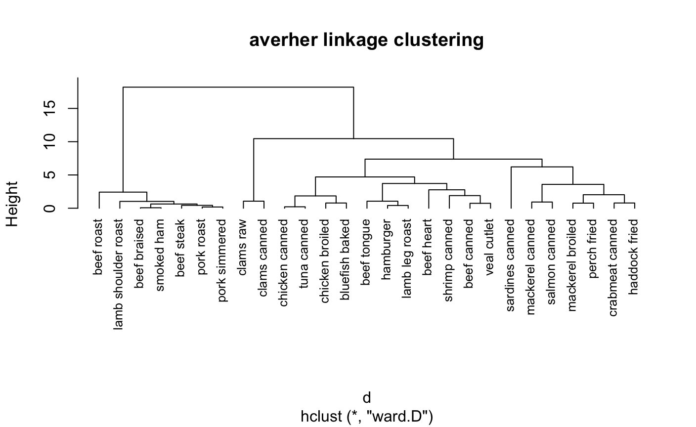
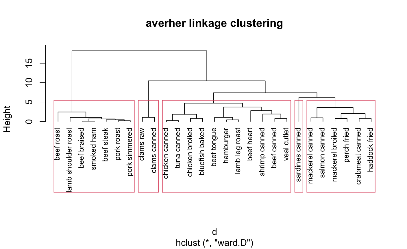
> ##########################聚类算法
> ####层次聚类
> par(mfrow = c(1,1))
> data(nutrient,package = "flexclust")
> row.names(nutrient)<-tolower(row.names(nutrient))
> #数据中心标准化scale()
> nutrient_s<-scale(nutrient,center = T)
> View(nutrient_s)
> #用dist()函数求出距离euclidean-欧几里得距离常用
> d<-dist(nutrient_s,method = "euclidean")
> #求出距离带入hclust函数中用ward方法聚类
> cnutrient<-hclust(d,method = "ward.D")
> plot(cnutrient,hang = -1,cex=.8,main='averher linkage clustering')
探究模型确定聚成几类合适
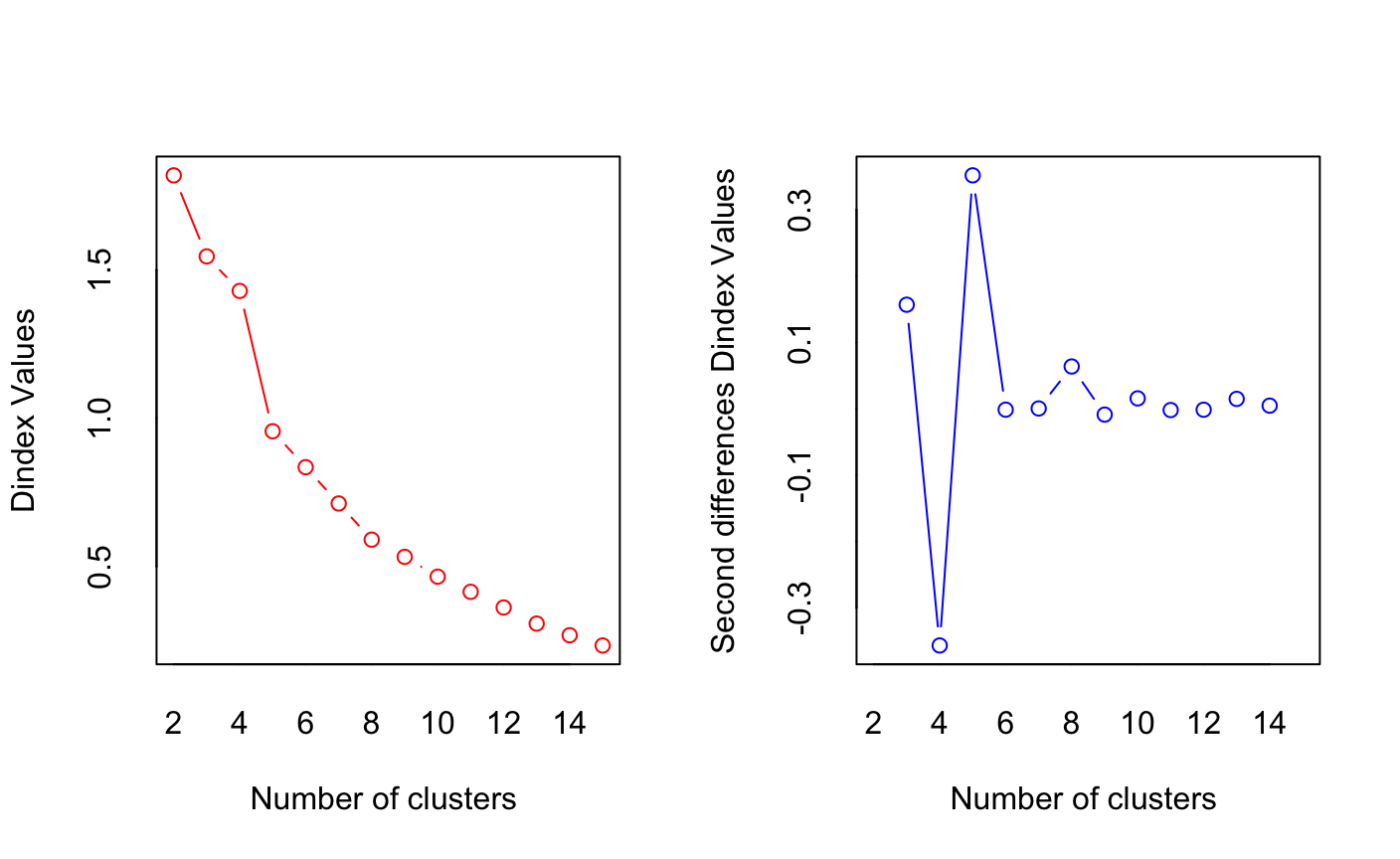
> ####用NbClust函数确定聚类K值
> library(NbClust)
> NC<-NbClust(nutrient_s,distance = "euclidean",min.nc = 2,max.nc = 15,method = "average")
> table(NC$Best.n[1,])

 0  1  2  3  4  5  9 10 13 14 15
 2  1  4  4  2  4  1  1  2  1  4
> barplot(table(NC$Best.n[1,]))
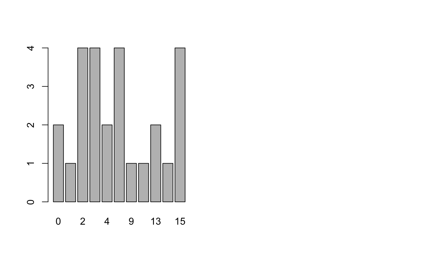
根据列表和柱状图我们可知聚为2、3、5、15类为不错的选项
下面我们看看聚为5类的结果
#####确定聚类个数后cut树
clusters<-cutree(cnutrient,k=5)
table(clusters)
plot(cnutrient,hang = -1,cex=.8,main='averher linkage clustering')
rect.hclust(cnutrient,k=5)
因为层次聚类计算距离非常复杂,所以能计算较小是数据集
K-Means聚类
1、选k个聚类中心点(随机生成)
2、把每个样本划分到距离最近的中心点
3、更新每类的中心点(可以把类的质心作为中心点)
4、重复2、3步骤,直至数据收敛
> #############k-means聚类
> data(wine,package = "rattle")
> head(wine,3)
  Type Alcohol Malic  Ash Alcalinity Magnesium Phenols Flavanoids Nonflavanoids
1    1   14.23  1.71 2.43       15.6       127    2.80       3.06          0.28
2    1   13.20  1.78 2.14       11.2       100    2.65       2.76          0.26
3    1   13.16  2.36 2.67       18.6       101    2.80       3.24          0.30
  Proanthocyanins Color  Hue Dilution Proline
1            2.29  5.64 1.04     3.92    1065
2            1.28  4.38 1.05     3.40    1050
3            2.81  5.68 1.03     3.17    1185
> df<-scale(wine[,-1],center = T)
> #确定聚类个数
> library(NbClust)
> nck<-NbClust(df,distance = "euclidean",min.nc = 2,max.nc = 15,method = "kmeans")

> table(nck$Best.n[1,])

 0  1  2  3 14 15
 2  1  2 19  1  1
> barplot(table(nck$Best.n[1,]))

从数据和图像可知聚为3类最好。
下面进行聚类:
> #kmeans输出详解
> #cluster:样本归属群号的向量
> #centers:聚类中心的矩阵,每一条记录,代表相应聚类的中心点
> #totss:所有数据的平方和
> #withinss:群内样本点进行scale(x,scale=F)后的平方和
> #tot.withinss:对所有群withinss的汇总
> #betweenss:totss与tot.withinss的差
> #size:每个群中的样本个数
> #iter:迭代的次数
> #ifault:指示可能的算法问题(专家使用),比如当一些点非常靠近的时候,算法也许不会收敛,就会返回ifault=4
> set.seed(1234)
> dfk<-kmeans(df,3,nstart = 25)
> #每类的大小
> dfk$size
[1] 62 65 51
> dfk$cluster
  [1] 1 1 1 1 1 1 1 1 1 1 1 1 1 1 1 1 1 1 1 1 1 1 1 1 1 1 1 1 1 1 1 1 1 1 1 1 1 1 1 1 1 1 1
 [44] 1 1 1 1 1 1 1 1 1 1 1 1 1 1 1 1 2 2 3 2 2 2 2 2 2 2 2 2 2 2 1 2 2 2 2 2 2 2 2 2 3 2 2
 [87] 2 2 2 2 2 2 2 2 2 1 2 2 2 2 2 2 2 2 2 2 2 2 2 2 2 2 2 2 2 2 2 2 3 2 2 1 2 2 2 2 2 2 2
[130] 2 3 3 3 3 3 3 3 3 3 3 3 3 3 3 3 3 3 3 3 3 3 3 3 3 3 3 3 3 3 3 3 3 3 3 3 3 3 3 3 3 3 3
[173] 3 3 3 3 3 3
> dfk$centers
     Alcohol      Malic        Ash Alcalinity   Magnesium     Phenols  Flavanoids
1  0.8328826 -0.3029551  0.3636801 -0.6084749  0.57596208  0.88274724  0.97506900
2 -0.9234669 -0.3929331 -0.4931257  0.1701220 -0.49032869 -0.07576891  0.02075402
3  0.1644436  0.8690954  0.1863726  0.5228924 -0.07526047 -0.97657548 -1.21182921
  Nonflavanoids Proanthocyanins      Color        Hue   Dilution    Proline
1   -0.56050853      0.57865427  0.1705823  0.4726504  0.7770551  1.1220202
2   -0.03343924      0.05810161 -0.8993770  0.4605046  0.2700025 -0.7517257
3    0.72402116     -0.77751312  0.9388902 -1.1615122 -1.2887761 -0.4059428
> table(dfk$cluster,wine$Type)#table(x,y)

     1  2  3
  1 59  3  0
  2  0 65  0
  3  0  3 48
聚类结果可视化
> ##进行绘图
> library(ggplot2)
> #factoextra包中fviz_nbclust可以确定最佳簇数,fviz_cluster画出聚类图
> library(factoextra)
> fviz_nbclust(df,kmeans,method = "silhouette")
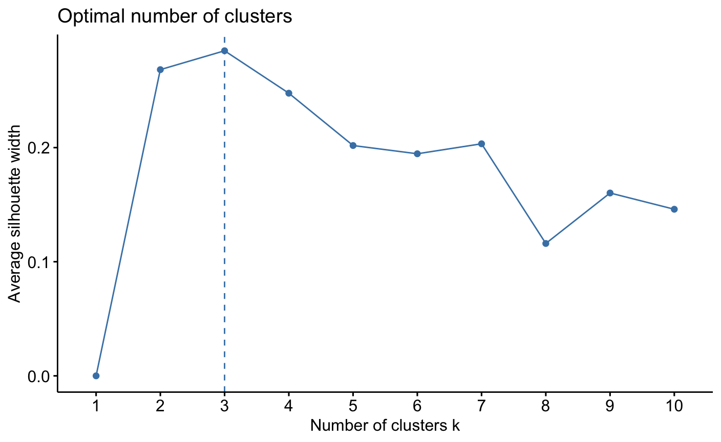
fviz_cluster(dfk, df, ellipse.type = "norm")
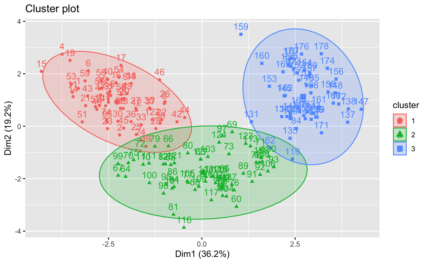
kmeans算法优点:有效率,而且不容易受初始值选择的影响
缺点:不能处理非球形簇,对离群值敏感。
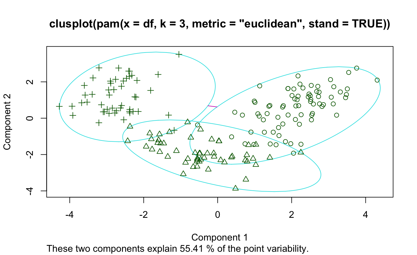
PAM
> ####k中心点PAM聚类
> library(cluster)
> set.seed(12)
> kp<-pam(df,k=3,metric="euclidean",stand = TRUE)
> table(kp$clustering,wine$Type)

     1  2  3
  1 59 16  0
  2  0 53  1
  3  0  2 47
> kp$medoids
        Alcohol      Malic        Ash Alcalinity   Magnesium    Phenols    Flavanoids
[1,]  0.5904981 -0.4711544  0.1584986  0.3009543  0.01809398  0.6469393  0.9518166597
[2,] -0.9246039 -0.5427655 -0.8985684 -0.1482061 -1.38222271 -1.0307762  0.0007311716
[3,]  0.4919549  1.4086355  0.4136527  1.0495551  0.15812565 -0.7911025 -1.2807313808
     Nonflavanoids Proanthocyanins       Color        Hue   Dilution      Proline
[1,]   -0.81841060      0.47016154  0.01807806  0.3611585  1.2089101  0.549706678
[2,]    0.06545479      0.06831575 -0.71522236  0.1861586  0.7863692 -0.752263054
[3,]    0.54756319     -0.31605849  0.96705508 -1.1263406 -1.4812670  0.009865569
> par(mfrow=c(1,1))
> clusplot(kp)