> ############################################线性回归
> setwd("/Users/yaozhilin/Downloads/R_edu/data")
> creditcard_exp<-read.csv("creditcard_exp.csv")
> head(creditcard_exp,3)
  id Acc avg_exp avg_exp_ln gender Age   Income Ownrent Selfempl dist_home_val
1 19   1 1217.03   7.104169      1  40 16.03515       1        1         99.93
2  5   1 1251.50   7.132098      1  32 15.84750       1        0         49.88
3 95   0      NA         NA      1  36  8.40000       0        0         88.61
  dist_avg_income age2   high_avg edu_class
1        15.93279 1600 0.10236053         3
2        15.79632 1024 0.05118421         2
3         7.49000 1296 0.91000000         1
> attach(creditcard_exp)
> lm<-lm(avg_exp~Income)
> summary(lm)

Call:
lm(formula = avg_exp ~ Income)

Residuals:
    Min      1Q  Median      3Q     Max
-608.11 -215.85  -82.69  202.90  772.50

Coefficients:
            Estimate Std. Error t value Pr(>|t|)
(Intercept)   258.05     104.29   2.474   0.0158 *
Income         97.73      12.99   7.524  1.6e-10 ***
---
Signif. codes:  0 ‘***’ 0.001 ‘**’ 0.01 ‘*’ 0.05 ‘.’ 0.1 ‘ ’ 1

Residual standard error: 332.1 on 68 degrees of freedom
  (30 observations deleted due to missingness)
Multiple R-squared:  0.4543,    Adjusted R-squared:  0.4463
F-statistic: 56.61 on 1 and 68 DF,  p-value: 1.603e-10
多元线型回归
#####多元线性回归
> #探究平均支出与年龄和收入等的线型关系
> lm_m<-lm(avg_exp~Age+Income+dist_avg_income+dist_home_val)
> coef(lm_m)
    (Intercept)             Age          Income dist_avg_income   dist_home_val
     -32.007774        1.372317     -166.720391      261.882708        1.532862
线型回归模型中的截距intercept一般忽略,现实中很少有数据都为零的实例,看income与avg_exp为负相关,我们仔细想想是不合逻辑的,后面肯定得调整。
> summary(lm_m)

Call:
lm(formula = avg_exp ~ Age + Income + dist_avg_income + dist_home_val)

Residuals:
    Min      1Q  Median      3Q     Max
-504.07 -208.81  -40.92  129.69  681.02

Coefficients:
                Estimate Std. Error t value Pr(>|t|)
(Intercept)      -32.008    186.874  -0.171  0.86454
Age                1.372      5.605   0.245  0.80735
Income          -166.720     87.607  -1.903  0.06147 .
dist_avg_income  261.883     87.807   2.982  0.00402 **
dist_home_val      1.533      1.057   1.450  0.15177
---
Signif. codes:  0 ‘***’ 0.001 ‘**’ 0.01 ‘*’ 0.05 ‘.’ 0.1 ‘ ’ 1

Residual standard error: 311.3 on 65 degrees of freedom
  (30 observations deleted due to missingness)
Multiple R-squared:  0.5416,    Adjusted R-squared:  0.5134
F-statistic:  19.2 on 4 and 65 DF,  p-value: 1.823e-10
看看自变量的显著值,age为0.807,dist_home_val为0.15都不显著,而且R2为0.54,调整R2为0.51,相差还是挺大的,所以后续考虑删除和合并一些变量
自变量的筛选
变量筛选有向前逐步法、向后逐步法、向前向后逐步法。衡量某一变量是否筛选在R中看指标AIC,AIC越小,模型越稳健。
> ###用向前向后逐步法筛选自变量
> #direction = c("both", "backward", "forward")
> lm_ms<-step(lm_m,direction = "both")
Start:  AIC=808.53
avg_exp ~ Age + Income + dist_avg_income + dist_home_val

                  Df Sum of Sq     RSS    AIC
- Age              1      5810 6306104 806.60
<none>                         6300294 808.53
- dist_home_val    1    203889 6504183 808.76
- Income           1    351031 6651325 810.33
- dist_avg_income  1    862197 7162491 815.51

Step:  AIC=806.6
avg_exp ~ Income + dist_avg_income + dist_home_val

                  Df Sum of Sq     RSS    AIC
<none>                         6306104 806.60
- dist_home_val    1    205826 6511930 806.85
- Income           1    345396 6651501 808.33
+ Age              1      5810 6300294 808.53
- dist_avg_income  1    857139 7163244 813.52
我们用到step函数,direction=“both”表示向前向后逐步法,我们看看程序是怎么运行筛选变量的。
Start: AIC=808.53,第一步放入所有的变量AIC=808.53
然后我们尝试去掉每一个变量看看AIC的值,发现去掉年龄时AIC最小为806.6,所以我们把Age去掉
第三步我们再次去掉其他的值看看AIC是否下降,并且尝试加上Age看看AIC的值,发现都不如去掉Age时AIC的值小
线型回归模型的诊断
模型已经进行了初步的变量筛选,但远远没有达到建模要求,我们需要对模型进行诊断。
我线性回归理论中提到,最小二乘求得的线性回归模型是有六大假设条件的:
- Y的平均值能够准确地被由X组成的线性函数建模出来。
- 解释变量之间不存在线性关系(或强相关)。
- 解释变量和随机扰动项不存在线性关系。
- 假设随机扰动项是一个均值为0的正态分布。
- 假设随机扰动项的方差恒为定
- 假设随机扰动项是独立的。
我们现在主要检测残差是否符合假设
#####线性回归的诊断
###残差检验
cre<-na.omit(creditcard_exp)
lm<-lm(avg_exp~Income)
summary(lm)
cre$pred<-predict(lm)
cre$res<-resid(lm)
plot(cre$res~cre$pred)#呈现喇叭口形状,说明异方差,可以用lny尝试
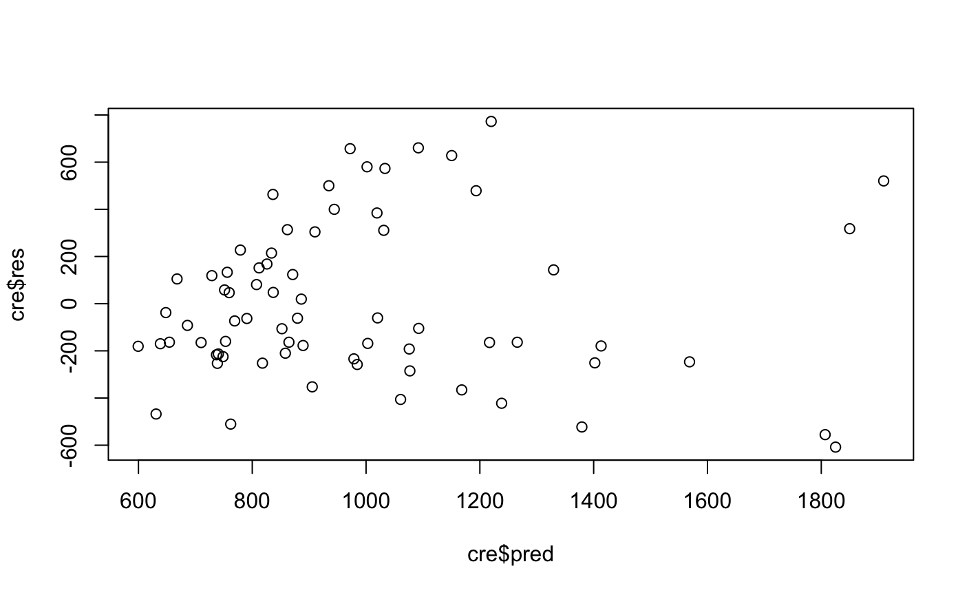
> library(lmtest)
> bptest(lm)#检验残差是否显著

    studentized Breusch-Pagan test

data:  lm
BP = 12.467, df = 1, p-value = 0.0004142
看得出结果是显著的
> #用lny调整残差存在异方差的模型
> lm1<-lm(avg_exp_ln~Income)
> summary(lm1)

Call:
lm(formula = avg_exp_ln ~ Income)

Residuals:
     Min       1Q   Median       3Q      Max
-1.33858 -0.21063 -0.03193  0.24935  0.61969

Coefficients:
            Estimate Std. Error t value Pr(>|t|)
(Intercept)  6.05875    0.11634  52.077  < 2e-16 ***
Income       0.09819    0.01449   6.776 3.58e-09 ***
---
Signif. codes:  0 ‘***’ 0.001 ‘**’ 0.01 ‘*’ 0.05 ‘.’ 0.1 ‘ ’ 1

Residual standard error: 0.3705 on 68 degrees of freedom
  (30 observations deleted due to missingness)
Multiple R-squared:  0.4031,    Adjusted R-squared:  0.3943
F-statistic: 45.92 on 1 and 68 DF,  p-value: 3.578e-09

> cre$pred1<-predict(lm1)
> cre$res1<-resid(lm1)
> library(lmtest)
> bptest(lm1)

    studentized Breusch-Pagan test

data:  lm1
BP = 0.60895, df = 1, p-value = 0.4352

> plot(cre$res1~cre$pred1)
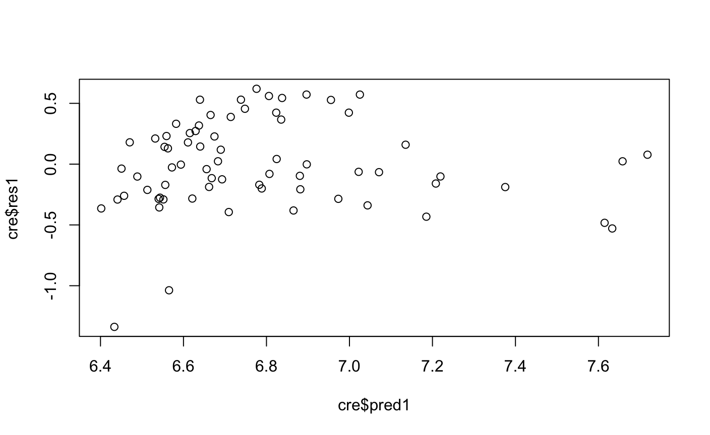
lny~x表示x每变化一个单位,y变化一个百分点,但从模型来看R2变为了0.40,比之前y~x的模型下降了,说明这模型解释是无理的。我们接下来继续探索。
> #用logy、logx调整残差存在异方差的模型
> cre$Income_log<-log(cre$Income)
> lm2<-lm(cre$avg_exp_ln~cre$Income_log)
> summary(lm2)

Call:
lm(formula = cre$avg_exp_ln ~ cre$Income_log)

Residuals:
     Min       1Q   Median       3Q      Max
-1.16234 -0.20937 -0.01781  0.27643  0.55853

Coefficients:
               Estimate Std. Error t value Pr(>|t|)
(Intercept)      5.0611     0.2217  22.833  < 2e-16 ***
cre$Income_log   0.8932     0.1126   7.929 2.95e-11 ***
---
Signif. codes:  0 ‘***’ 0.001 ‘**’ 0.01 ‘*’ 0.05 ‘.’ 0.1 ‘ ’ 1

Residual standard error: 0.3457 on 68 degrees of freedom
Multiple R-squared:  0.4804,    Adjusted R-squared:  0.4728
F-statistic: 62.87 on 1 and 68 DF,  p-value: 2.95e-11

> cre$pred2<-predict(lm2)
> cre$res2<-resid(lm2)
> plot(cre$res2~cre$pred2)
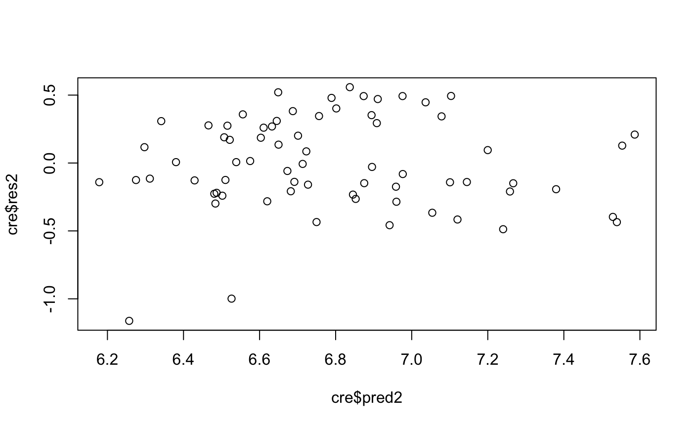
看结果已经完全消除了异方差现象,但有人会疑问,lnx和lny不是线性关系,其实x和y都是到手的数据,我们可以随意的变化。
消除强影响点
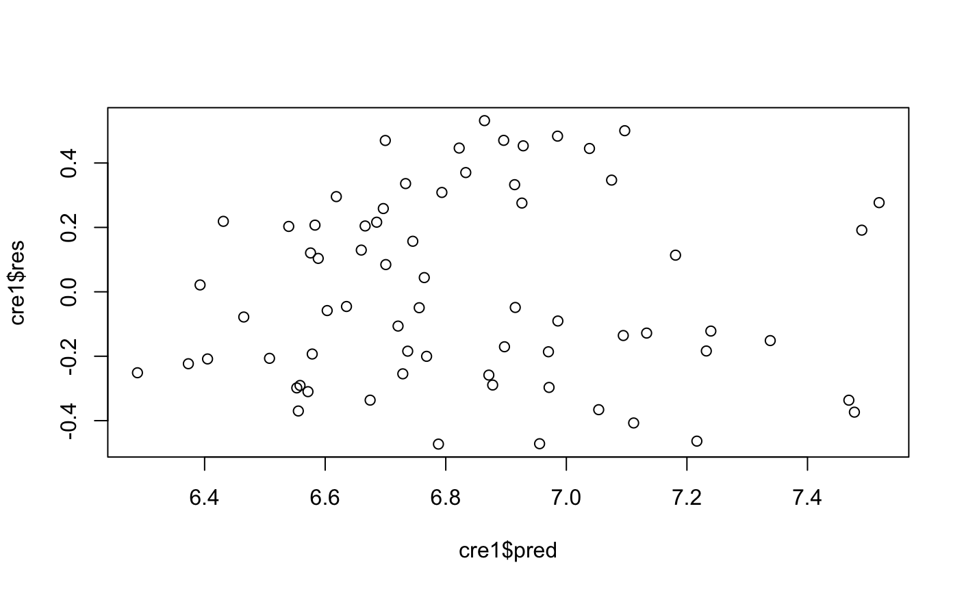
> #学生化残差消除强影响点
> cre$res_t<-(cre$res2-mean(cre$res2))/sd(cre$res2)
> #选出95%的值
> cre1<-subset(cre,abs(res_t)<=2)
> lm3<-lm(cre1$avg_exp_ln~cre1$Income_log)
> summary(lm3)

Call:
lm(formula = cre1$avg_exp_ln ~ cre1$Income_log)

Residuals:
     Min       1Q   Median       3Q      Max
-0.47280 -0.23028 -0.05378  0.22875  0.53152

Coefficients:
                Estimate Std. Error t value Pr(>|t|)
(Intercept)      5.31234    0.19249  27.598  < 2e-16 ***
cre1$Income_log  0.78040    0.09723   8.027 2.37e-11 ***
---
Signif. codes:  0 ‘***’ 0.001 ‘**’ 0.01 ‘*’ 0.05 ‘.’ 0.1 ‘ ’ 1

Residual standard error: 0.2911 on 66 degrees of freedom
Multiple R-squared:  0.494,    Adjusted R-squared:  0.4863
F-statistic: 64.43 on 1 and 66 DF,  p-value: 2.372e-11

> cre1$pred<-predict(lm3)
> cre1$res<-resid(lm3)
> plot(cre1$res~cre1$pred)
多重共线性的检测
> ###多重共线性的检测
> lm4<-lm(avg_exp~Age+Income+dist_avg_income+dist_home_val)
> lm5<-step(lm4,direction = "both")
Start:  AIC=808.53
avg_exp ~ Age + Income + dist_avg_income + dist_home_val

                  Df Sum of Sq     RSS    AIC
- Age              1      5810 6306104 806.60
<none>                         6300294 808.53
- dist_home_val    1    203889 6504183 808.76
- Income           1    351031 6651325 810.33
- dist_avg_income  1    862197 7162491 815.51

Step:  AIC=806.6
avg_exp ~ Income + dist_avg_income + dist_home_val

                  Df Sum of Sq     RSS    AIC
<none>                         6306104 806.60
- dist_home_val    1    205826 6511930 806.85
- Income           1    345396 6651501 808.33
+ Age              1      5810 6300294 808.53
- dist_avg_income  1    857139 7163244 813.52
> library(car)
> vif(lm5)#膨胀因子大于10时共线性问题就比较严重
         Income dist_avg_income   dist_home_val
      51.176222       51.610836        1.084867
可以看出共线性的问题还是比较严重的,后续我会尝试用变量聚类,因子分析或者正则化方法消除共线性问题。