手写数字识别经典案例,旨在熟悉cnn网络结构,掌握tf编写cnn的方法。
# encoding:utf-8
import tensorflow as tf
import input_data

# 自动下载安装数据集
mnist = input_data.read_data_sets("MNIST_data/", one_hot=True)
x=tf.placeholder('float',[None,784])        # None 为样本个数   784=28*28

### 初始化权重和偏置
# 一般来说初始化权重时要加入少量扰动,打破对称性,防止0梯度的问题。
# Relu要用稍大于0的值,避免节点输出恒为0
def weight_variable(shape):
    initial = tf.truncated_normal(shape, stddev=0.1)    # 截断的正态分布
    return tf.Variable(initial)

def bias_variable(shape):
    initial = tf.constant(0.1, shape=shape)     # 经验:取正数较好
    return tf.Variable(initial)

### 卷积和池化
def conv2d(x, W):
    # 卷积
    # stride [1, x_movement, y_movement, 1]    步长,长度必须是4
    # Must have strides[0] = strides[3] = 1
    # padding 取same时卷积后的长宽和原图片一样,此时需要对原图片进行边界填充
    return tf.nn.conv2d(x, W, strides=[1, 1, 1, 1], padding='SAME')

def max_pool_2x2(x):
    # 池化
    # ksize 是池化视野的大小 2x2
    # strides padding 与卷积不同,取same时可能对原样本进行填充,注意是可能,且不要求和原样本大小一样,应该是一定不一样
    return tf.nn.max_pool(x, ksize=[1, 2, 2, 1], strides=[1, 2, 2, 1], padding='SAME')

## 第一层卷积
# 权重就是卷积核,前两个维度是patch的大小,接着是输入的通道数目(或者说卷积核的通道数),最后是输出的通道数目(或者说卷积核的个数)
W_conv1 = weight_variable([5, 5, 1, 32])    # 卷积核个数一般取2的n次方,n不限
# 输出对应一个同样大小的偏置向量
b_conv1 = bias_variable([32])       # 一个卷积核一个w,一个w一个b,故几个卷积核几个b

# 把x变成一个4d向量,第1维是样本个数,-1代表暂时不确定,2 3维代表图片的宽高,最后一维是颜色通道(本例是黑白图片)
x_image = tf.reshape(x, [-1, 28, 28, 1])

# 把x_image和权值向量进行卷积相乘,加上偏置,使用relu函数激活,最后max pooling
h_conv1 = tf.nn.relu(conv2d(x_image, W_conv1) + b_conv1)
h_pool1 = max_pool_2x2(h_conv1)

# 这层卷积完图片为  28*28*32    长宽不变,深度加深
# 这层池化完图片为 14*14*32     池化视野2x2,步长2,2

## 第二层卷积
# 为了构建更深的网络,我们把几个类似的层堆叠起来
W_conv2 = weight_variable([5, 5, 32, 64])       # 32 是第一层卷完的深度(通道数) 64继续加深
b_conv2 = bias_variable([64])

h_conv2 = tf.nn.relu(conv2d(h_pool1, W_conv2) + b_conv2)
h_pool2 = max_pool_2x2(h_conv2)

# 这层卷积完图片为 14*14*64
# 这层池化完图片为 7*7*64

## 全连接层
# 这时图片的维度降到7x7, 加入一个有1024个神经元的全连接层,用于处理整个图片
W_fc1 = weight_variable([7 * 7 * 64, 1024])     # 全连接层此时的权重是2维的,即上次神经元个数,下层神经元个数
b_fc1 = bias_variable([1024])

# 我们把池化层输出的张量reshape成一维向量,乘以权重,加上偏置,激活
h_pool2_flat = tf.reshape(h_pool2, [-1, 7 * 7 * 64])            # 将图片展开(flat)变成1维向量, -1 仍代表样本个数
h_fc1 = tf.nn.relu(tf.matmul(h_pool2_flat, W_fc1) + b_fc1)

## dropout
# 为了减少过拟合,在输出层之前加上dropout
# 用一个placeholder来代表一个神经元在dropout中被保留的概率。
# 这样可以在训练过程中启用dropout,在测试过程中关闭dropout。
# tf.nn.dropout操作会自动处理神经元输出值的scale。所以用dropout的时候不用考虑scale
keep_prob = tf.placeholder('float')
h_fc1_drop = tf.nn.dropout(h_fc1, keep_prob)

## 输出层
# 最后添加softmax层
W_fc2 = weight_variable([1024, 10])
b_fc2 = bias_variable([10])

y_conv = tf.nn.softmax(tf.matmul(h_fc1_drop, W_fc2) + b_fc2)

# 损失函数
y_=tf.placeholder('float',[None,10])     # 10维
cross_entropy = -tf.reduce_sum(y_*tf.log(y_conv))

# 优化器
train_step = tf.train.AdamOptimizer(1e-4).minimize(cross_entropy)

# 评估
correct_prediction = tf.equal(tf.argmax(y_conv,1), tf.argmax(y_,1))
accuracy = tf.reduce_mean(tf.cast(correct_prediction, "float"))

# 训练
sess = tf.Session()
sess.run(tf.initialize_all_variables())

for i in range(20000):
    batch = mnist.train.next_batch(50)
    if i%100 == 0:
        train_accuracy = sess.run(accuracy, feed_dict={x: batch[0], y_: batch[1], keep_prob: 1.0})
        print "step %d, training accuracy %g"%(i, train_accuracy)
    sess.run(train_step, feed_dict={x: batch[0], y_: batch[1], keep_prob: 0.5})

print "test accuracy %g"%sess.run(accuracy, feed_dict={x: mnist.test.images, y_: mnist.test.labels, keep_prob: 1.0})
手写数字识别任务比较简单,据资料显示 2层卷积2层全连接的网络结构,是目前识别率最高的cnn模型。
对于复杂的场景
1. 通常需要更多的辅助技术,如集成学习,学习率衰减,数据扩充,
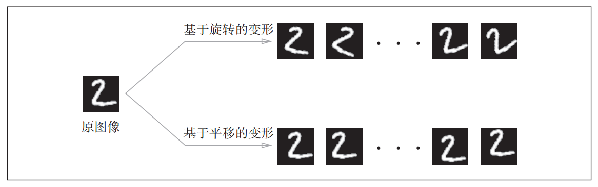
集成学习和lr衰减没什么好说的,这里简单介绍一下数据扩充。
数据扩充是基于某种算法人为的扩充训练集,如对图像进行旋转、平移等,这对数据集有限的情况非常有用。
还有比如 裁剪图像的crop处理,左右翻转的flip处理,增加亮度等外观变化,缩放等尺寸变化。
2. 也需要更深的网络和更复杂的结构,比如VGG,后面我会介绍。