# library
# standard library
import os
# third-party library
import torch
import torch.nn as nn
import torch.utils.data as Data
import torchvision
import matplotlib.pyplot as plt
# torch.manual_seed(1) # reproducible
# Hyper Parameters
EPOCH = 1 # train the training data n times, to save time, we just train 1 epoch
BATCH_SIZE = 50
LR = 0.001 # learning rate
DOWNLOAD_MNIST = False
# Mnist digits dataset
if not(os.path.exists('./mnist/')) or not os.listdir('./mnist/'):
# not mnist dir or mnist is empyt dir
DOWNLOAD_MNIST = True
train_data = torchvision.datasets.MNIST(
root='./mnist/',
train=True, # this is training data
transform=torchvision.transforms.ToTensor(), # Converts a PIL.Image or numpy.ndarray to
# torch.FloatTensor of shape (C x H x W) and normalize in the range [0.0, 1.0]
download=DOWNLOAD_MNIST,
)
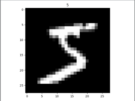
# plot one example 每个图片都是灰度图片,高度为1,长宽为28;RGB图片的高度为3。
print(train_data.train_data.size()) # (60000, 28, 28)
print(train_data.train_labels.size()) # (60000)
plt.imshow(train_data.train_data[0].numpy(), cmap='gray')
plt.title('%i' % train_data.train_labels[0])
plt.show()
# Data Loader for easy mini-batch return in training, the image batch shape will be (50, 1, 28, 28)
train_loader = Data.DataLoader(dataset=train_data, batch_size=BATCH_SIZE, shuffle=True)
# pick 2000 samples to speed up testing
test_data = torchvision.datasets.MNIST(root='./mnist/', train=False)
test_x = torch.unsqueeze(test_data.test_data, dim=1).type(torch.FloatTensor)[:2000]/255. # shape from (2000, 28, 28) to (2000, 1, 28, 28), value in range(0,1)
test_y = test_data.test_labels[:2000]
class CNN(nn.Module):
def __init__(self):
super(CNN, self).__init__()
self.conv1 = nn.Sequential( # input shape (1, 28, 28)
nn.Conv2d(
in_channels=1, # 灰度图片的高度为1,input height
out_channels=16, # 16个卷积,之后高度为从1变成6,长宽不变,n_filters
kernel_size=5, # 5*5宽度的卷积,filter size
stride=1, # 步幅为1,filter movement/step
padding=2, # 周围填充2圈0,if want same width and length of this image after Conv2d, padding=(kernel_size-1)/2 if stride=1
), # output shape (16, 28, 28)
nn.ReLU(), # 激活时,图片长宽高不变,activation
nn.MaxPool2d(kernel_size=2), # 4合1的池化,之后图片的高度不变,长宽减半,choose max value in 2x2 area, output shape (16, 14, 14)
)
self.conv2 = nn.Sequential( # input shape (16, 14, 14)
nn.Conv2d(16, 32, 5, 1, 2), # output shape (32, 14, 14)
nn.ReLU(), # activation
nn.MaxPool2d(2), # output shape (32, 7, 7)
)
self.out = nn.Linear(32 * 7 * 7, 10) # fully connected layer, output 10 classes
def forward(self, x):
x = self.conv1(x)
x = self.conv2(x) # 考虑bach之后的数据输出是(batch, 32, 7, 7)
x = x.view(x.size(0), -1) # 保持bach不变,将数据展开成一行的,flatten the output of conv2 to (batch_size, 32 * 7 * 7)
output = self.out(x)
return output, x # return x for visualization
cnn = CNN()
print(cnn) # net architecture
optimizer = torch.optim.Adam(cnn.parameters(), lr=LR) # optimize all cnn parameters
loss_func = nn.CrossEntropyLoss() # the target label is not one-hotted
# following function (plot_with_labels) is for visualization, can be ignored if not interested
from matplotlib import cm
try: from sklearn.manifold import TSNE; HAS_SK = True
except: HAS_SK = False; print('Please install sklearn for layer visualization')
def plot_with_labels(lowDWeights, labels):
plt.cla()
X, Y = lowDWeights[:, 0], lowDWeights[:, 1]
for x, y, s in zip(X, Y, labels):
c = cm.rainbow(int(255 * s / 9)); plt.text(x, y, s, backgroundcolor=c, fontsize=9)
plt.xlim(X.min(), X.max()); plt.ylim(Y.min(), Y.max()); plt.title('Visualize last layer'); plt.show(); plt.pause(0.01)
plt.ion()
# training and testing
for epoch in range(EPOCH):
for step, (b_x, b_y) in enumerate(train_loader): # gives batch data, normalize x when iterate train_loader
output = cnn(b_x)[0] # cnn output
loss = loss_func(output, b_y) # cross entropy loss
optimizer.zero_grad() # clear gradients for this training step
loss.backward() # backpropagation, compute gradients
optimizer.step() # apply gradients
if step % 50 == 0:
test_output, last_layer = cnn(test_x)
pred_y = torch.max(test_output, 1)[1].data.numpy()
accuracy = float((pred_y == test_y.data.numpy()).astype(int).sum()) / float(test_y.size(0))
print('Epoch: ', epoch, '| train loss: %.4f' % loss.data.numpy(), '| test accuracy: %.2f' % accuracy)
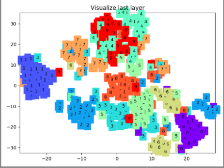
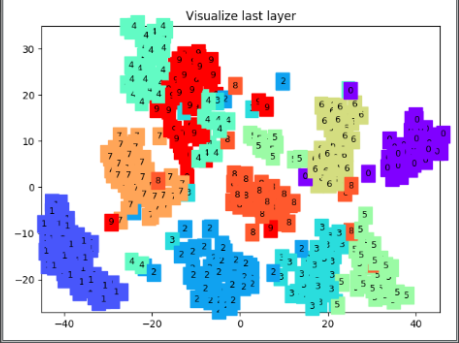
if HAS_SK:
# Visualization of trained flatten layer (T-SNE)
tsne = TSNE(perplexity=30, n_components=2, init='pca', n_iter=5000)
plot_only = 500
low_dim_embs = tsne.fit_transform(last_layer.data.numpy()[:plot_only, :])
labels = test_y.numpy()[:plot_only]
plot_with_labels(low_dim_embs, labels)
plt.ioff()
# print 10 predictions from test data
test_output, _ = cnn(test_x[:10])
pred_y = torch.max(test_output, 1)[1].data.numpy()
print(pred_y, 'prediction number')
print(test_y[:10].numpy(), 'real number')
打印网络结构
print(cnn)  # net architecture

> CNN(
>   (conv1): Sequential(
>     (0): Conv2d(1, 16, kernel_size=(5, 5), stride=(1, 1), padding=(2, 2))
>     (1): ReLU()
>     (2): MaxPool2d(kernel_size=2, stride=2, padding=0, dilation=1, ceil_mode=False)
>   )
>   (conv2): Sequential(
>     (0): Conv2d(16, 32, kernel_size=(5, 5), stride=(1, 1), padding=(2, 2))
>     (1): ReLU()
>     (2): MaxPool2d(kernel_size=2, stride=2, padding=0, dilation=1, ceil_mode=False)
>   )
>   (out): Linear(in_features=1568, out_features=10, bias=True)
> )
打印训练过程
Epoch:  0 | train loss: 2.3170 | test accuracy: 0.11
Epoch:  0 | train loss: 0.2893 | test accuracy: 0.83
Epoch:  0 | train loss: 0.4333 | test accuracy: 0.90
  .......
Epoch:  0 | train loss: 0.1268 | test accuracy: 0.98
从测试数据中打印10个预测
# print 10 predictions from test data
print(pred_y, 'prediction number')
print(test_y[:10].numpy(), 'real number')

> [7 2 1 0 4 1 4 9 5 9] prediction number
> [7 2 1 0 4 1 4 9 5 9] real number
END