壁虎书6 Decision Trees

　　Decision Trees are versatile Machine Learning algorithms that can perform both classification and regression tasks，and even multioutput tasks. Decision Trees are the fundamental components of Random Forests，which are among the most powerful Machine Learning algorithms available today. 

Training and Visualizing a Decision Tree: 

from sklearn.datasets import load_iris
from sklearn.tree import DecisionTreeClassifier
from sklearn.tree import export_graphviz  # 可视化

iris = load_iris()
X = iris.data[:, 2:]  # petal length and width
y = iris.target

tree_clf = DecisionTreeClassifier(max_depth=2)
tree_clf.fit(X, y)

export_graphviz(tree_clf,
                out_file='iris_tree.dot',
                feature_names=iris.feature_names[2:],
                class_names=iris.target_names,
                filled=True, 
                   rounded=True)

　　then convert this .dot file to a variety of formats such as PDF or PNG using the dot command-line tool from the graphviz package.

$ dot -Tpng iris_tree.dot -o iris_tree.png

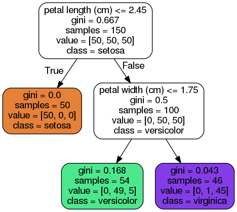
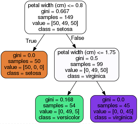
　　Figure 6-1 Iris Decision Tree

　　

　　几个属性：

　　　　class

　　　　samples

　　　　value: how many training instances of each class this node applies to: for example，the bottom-right node(vlaue=[0, 1, 45]) applies to 0 Iris-Setosa，1 Iris-Versicolor，and 45 Iris-Virginica. 

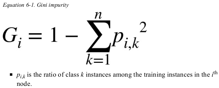
　　　　gini: measure its impurity，a node is “pure” (gini=0) if  all training instances it applies to belong to the same class，e.g., (depth 1，left). 

　　the approach to compute the gini score of the i-nd node: 

　　

　　以 (depth-2 left) 为例，

Making Predictions: 

　　从root node 开始，直到leaf node. 

　　one of the many qualities of Decision Trees is that they require very little data preparation. in particular，they don't require feature scaling or centering at all. 

　　Scikit-Learn uses the CART algorithm，which produces only binary tree. other algorithms such as ID3 can produce Decision Trees with nodes that have more than two children. 

　　

　　Figure 6-2 shows this Decision Tree's decision boundaries. the thick vertical line represents the decision boundary of the root node(depth 0): petal length = 2.45 cm. since the left area is pure，it can't be split any further. however，the right area is impure，so the depth-1 right node splits it at petal width = 1.75 cm. since max_depth was set to 2，the Decision Trees stops right there. if you set max_depth to 3，then the two depth-2 nodes would each add another decision boundary. 

import numpy as np
import matplotlib.pyplot as plt
from matplotlib.colors import ListedColormap
from sklearn.datasets import load_iris
from sklearn.tree import DecisionTreeClassifier

iris = load_iris()
X = iris.data[:, 2:]  # petal length and width
y = iris.target

tree_clf = DecisionTreeClassifier(max_depth=2, random_state=42)
tree_clf.fit(X, y)


def plot_decision_boundary(clf, X, y, axes=[0, 7.5, 0, 3], iris=True, legend=False, plot_training=True):
    x1s = np.linspace(axes[0], axes[1], 100)
    x2s = np.linspace(axes[2], axes[3], 100)
    x1, x2 = np.meshgrid(x1s, x2s)
    X_new = np.c_[x1.ravel(), x2.ravel()]
    y_pred = clf.predict(X_new).reshape(x1.shape)
    custom_cmap = ListedColormap(['#fafab0','#9898ff','#a0faa0'])
    plt.contourf(x1, x2, y_pred, alpha=0.3, cmap=custom_cmap)
    if not iris:
        custom_cmap2 = ListedColormap(['#7d7d58','#4c4c7f','#507d50'])
        plt.contour(x1, x2, y_pred, cmap=custom_cmap2, alpha=0.8)
    if plot_training:
        plt.plot(X[:, 0][y == 0], X[:, 1][y == 0], "yo", label="Iris-Setosa")
        plt.plot(X[:, 0][y == 1], X[:, 1][y == 1], "bs", label="Iris-Versicolor")
        plt.plot(X[:, 0][y == 2], X[:, 1][y == 2], "g^", label="Iris-Virginica")
        plt.axis(axes)
    if iris:
        plt.xlabel("Petal length", fontsize=14)
        plt.ylabel("Petal width", fontsize=14)
    else:
        plt.xlabel(r"$x_1$", fontsize=18)
        plt.ylabel(r"$x_2$", fontsize=18, rotation=0)
    if legend:
        plt.legend(loc="lower right", fontsize=14)


plt.figure(figsize=(8, 4))
plot_decision_boundary(tree_clf, X, y)
plt.plot([2.45, 2.45], [0, 3], "k-", linewidth=2)
plt.plot([2.45, 7.5], [1.75, 1.75], "k--", linewidth=2)
plt.plot([4.95, 4.95], [0, 1.75], "k:", linewidth=2)
plt.plot([4.85, 4.85], [1.75, 3], "k:", linewidth=2)
plt.text(1.40, 1.0, "Depth=0", fontsize=15)
plt.text(3.2, 1.80, "Depth=1", fontsize=13)
plt.text(4.05, 0.5, "(Depth=2)", fontsize=11)
plt.show()

　　

Model Interpretation: white box versus black box: 

　　Decision Trees are fairly intuitive and their decisions are easy to interpret. such models are often called white box models. in contrast，Random Forests or neural networks are generally considered black box models. 

Estimating Class Probabilities: 

　　a Decision Tree can also estimate the probability that an instance belongs to a particular class k: first it traverses the tree to find the leaf node for this instance，and then it returns the ratio of training instances of class k in this node.  for example，suppose you have found a flower whose petals are 5cm long and 1.5cm wide. the corresponding leaf node is the depth-2 left node，so the Decision Tree should output the following probabilities: 0% for Iris-Setosa(0/ 54)，90.7% for Iris-Versicolor(49/54)，and 9.3% for Iris-Virginica(5/54). if you ask it to predict the class，it should output Iris-Versicolor(class 1) since it has the highest probability. 

print(tree_clf.predict_proba([[5, 1.5]]))  # [[0.         0.90740741 0.09259259]]
print(tree_clf.predict([[5, 1.5]]))  # [1]

The CART Training Algorithm: 

　　Scikit-Learn uses the Classification And Regression Tree(CART) algorithm to train Decision Tree. the idea is really simple: the algorithm first splits the training set in two subsets using a single feature k and a threshold t_k (e.g., petal length ≤ 2.45 cm). 

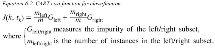
　　the approach to choose k and t_k : it search for the pair(k, t_k) that produces the purest subsets(weighted by their size). 

　　the cost function that the algorithm tries to minimize is given by Equation 6-2: 

　　

　　once it has successfully split the training set in two，it splits the subsets using the same logic，then the sub-subsets and so on，recursively. it stops recursing once it reaches the maximum depth(max_depth hyperparameter)，or if it can't find a split that reduce impurity. a few other hyperparameters conditions(min_samples_split，min_samples_leaf，min_weight_fraction_leaf，and max_leaf_nodes). 

　　the CART algorithm is a greedy algorithm: it greedily searches for an optimum split at the top level，then repeats the process at each level. it doesn't check whether or not the split will lead to the lowest possible impurity several level down. a greedy algorithm often produces a reasonably good solution，but it is not guaranteed to be the optimal solution. 

　　unfortunately，finding the optimal tree is known to be an NP-Complete problem. it  requires O(exp(m)) time，making the problem intractable even for fairly small training sets. 

Computational Complexity: 

　　making predictions requires traversing the Decision Tree from the root to a leaf. Decision Trees are generally approximately balanced，so traversing the Decision Tree requires going through roughly O(log₂(m)) nodes. since each node only requires checking the value of one feature，the overall prediction complexity is just O(log₂(m))，independent of the number of features. so predictions are very fast，even when dealing with large training sets. 

　　however，the training algorithm compares all features(or less if max_features is set) on all samples at each node. this result in a training complexity of O(n × mlog(m)). 

　　for small training sets(less than a few thousand instances)，Scikit-Learn can speed up training by presorting the data(set presort=True)，but this slows down training considerably for larger training sets. 

Gini Impurity or Entropy?

　　by default，the Gini impurity measure is used，but you can select the entropy impurity measure instead by setting criterion hyperparameter to “entropy”.

　　the concept of entropy originated in thermodynamics as a measure of molecular disorder: entropy approaches zero when molecules are still and well ordered. it later spread to a wide variety of domains，including Shannon's information theory，where it measures the average information content of a message: entropy is zero when all messages are identical. in Machine learning，it is frequently used as an impurity measure: a set's entropy is zero when it contains instances of only one class. 

　　Equation 6-3 shows the definition of the entropy of the i^th node.

　　

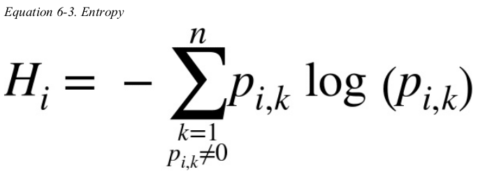
　　for example，the depth-2 left node in Figure 6-1 has an entropy equal to .

　　so should you use Gini impurity or entropy？the truth is，most of the time it doesn't make a big difference: they lead to similar trees. Gini impurity is slightly faster to compute，so it is a good default. however，when they differ，Gini impurity tends to isolate the most frequent class in its  own branch of the tree，while entropy tends to produce slightly more balanced trees. 

Regularization Hyperparameters: 

　　Decision Trees make very few assumptions about the training data. if left unconstrained，the tree structure will adapt itself to the training data，fitting it very closely，and most likely overfitting it. such a model is often called a nonparametric model，not because it doesn't have any parameters (it often has a lot) but because the number of parameters isn't determined prior to training，so the model structure is free to stick closely to the data. 注意：是参数个数不确定，而不是参数本身。

　　in contrast，a parametric model such as a linear model has a predetermined number of parameters，so its degree of freedom is limited，reducing the risk of overfitting (but increasing the risk of underfitting). 

　　to avoid overfitting the training data，you need to restrict the Decision Tree's freedom during training. 即regularization。

　　the regularization hyperparameters depend on the algorithm used，but generally you can at least restrict the maximum depth of the Decision Tree. in Scikit-learn，this is controlled by the max_depth hyperparameter(the default value is None，which means unlimited). reducing max_depth will regularize the model and thus reduce the risk of overfitting. 

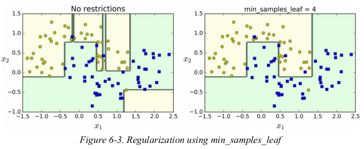
　　the DecisionTreeClassifier class has a few other parameters that similarly restrict the shape of the Decision Tree: min_samples_split (the minimum number of samples a node must have before it can be split)，min_samples_leaf (the minimum number of samples a leaf node must have)，min_weight_fraction_leaf (same as min_samples_leaf but expressed as a fraction of the total number of weighted instances)，max_leaf_nodes (maximum number of leaf nodes)，max_features (maximum number of features that are evaluated for splitting at each node). 

　　increasing min_* or reducing max_* hyperparameters will regularize the model. 

import numpy as np
import matplotlib.pyplot as plt
from matplotlib.colors import ListedColormap
from matplotlib.colors import ListedColormap
from sklearn.datasets import make_moons
from sklearn.tree import DecisionTreeClassifier

X, y = make_moons(n_samples=100, noise=0.25, random_state=53)

deep_tree_clf1 = DecisionTreeClassifier(random_state=42)
deep_tree_clf2 = DecisionTreeClassifier(min_samples_leaf=4, random_state=42)
deep_tree_clf1.fit(X, y)
deep_tree_clf2.fit(X, y)


def plot_decision_boundary(clf, X, y, title, axes=[-1.5, 2.5, -1.0, 1.5]):
    x1s = np.linspace(axes[0], axes[1], 100)
    x2s = np.linspace(axes[2], axes[3], 100)
    x1, x2 = np.meshgrid(x1s, x2s)
    X_new = np.c_[x1.ravel(), x2.ravel()]
    y_pred = clf.predict(X_new).reshape(x1.shape)  # shape要一致
    custom_cmap = ListedColormap(['#fafab0', '#9898ff', '#a0faa0'])
    plt.contourf(x1, x2, y_pred, alpha=0.3, cmap=custom_cmap)

    plt.plot(X[:, 0][y == 0], X[:, 1][y == 0], "yo", label="Iris-Setosa")
    plt.plot(X[:, 0][y == 1], X[:, 1][y == 1], "bs", label="Iris-Versicolor")
    plt.plot(X[:, 0][y == 2], X[:, 1][y == 2], "g^", label="Iris-Virginica")
    plt.axis(axes)
    plt.title(title)
    plt.xlabel('$x_1$', fontsize=14)
    plt.ylabel('$x_2$', rotation=0, fontsize=14)


plt.figure(figsize=(11, 4))
plt.subplot(121)  # 设置子图一定是在所有子图操作之前进行
plot_decision_boundary(deep_tree_clf1, X, y, 'No restrictions')
plt.subplot(122)
plot_decision_boundary(deep_tree_clf2, X, y, 'min_samples_leaf = {}'.format(deep_tree_clf2.min_samples_leaf))
plt.show()

　　

　　other algorithms work by first training the Decision Tree without restrictions，then pruning (deleting) unnecessary nodes. a node whose children are all leaf nodes is considered unnecessary if the purity improvement it provides is not statistically significant. standard statistical tests，such as 卡方检验，are used to estimate the probability that the improvement is purely the result of chance (which is called the null hypothesis). if this probability，called the p-value，is higher than a given threshold (typically 5%，controlled by a hyperparameter)，then the node is considered unnecessary and its children are deleted. the pruning continues until all unnecessary nodes have been pruned. 

Regression: 

　　Decision Trees are also capable of performing regression tasks. 

from sklearn.tree import DecisionTreeRegressor
from sklearn.tree import export_graphviz

np.random.seed(42)
m = 200
X = np.random.rand(m, 1)
y = 4 * (X - 0.5) ** 2 + np.random.randn(m, 1) / 10

tree_reg = DecisionTreeRegressor(max_depth=2)
tree_reg.fit(X, y)

export_graphviz(tree_reg,
                out_file='tree_reg.dot',
                feature_names=['x1'],
                rounded=True,
                filled=True)

　　

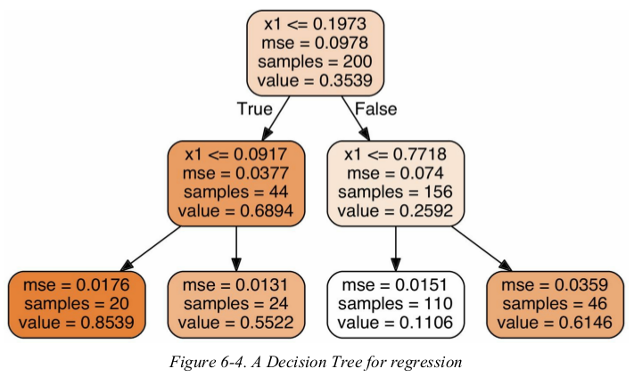
　　this tree looks very similar to the classification tree you built earlier. the main difference is that instead of predicting a class in each node，it predicts a value. for example，suppose you want to make a prediction for a new instance with x₁ = 0.6. you traverses the tree starting at the root，and eventually reach the leaf node that predicts value=0.1106. this prediction is simply the average target value of the 110 training instances associated to this leaf node. this prediction results in a Mean Squared Error (MSE) equal to 0.0151 over these 110 instances. 

import numpy as np
import matplotlib.pyplot as plt
from sklearn.tree import DecisionTreeRegressor

np.random.seed(42)
m = 200
X = np.random.rand(m, 1)
y = 4 * (X - 0.5) ** 2 + np.random.randn(m, 1) / 10

tree_reg1 = DecisionTreeRegressor(random_state=42, max_depth=2)
tree_reg2 = DecisionTreeRegressor(random_state=42, max_depth=3)
tree_reg1.fit(X, y)
tree_reg2.fit(X, y)


def plot_regression_predictions(tree_reg, X, y, axes=[0, 1, -0.2, 1], ylabel='$y$'):
    x1 = np.linspace(axes[0], axes[1], 500).reshape(-1, 1)
    y_pred = tree_reg.predict(x1)
    plt.axis(axes)
    plt.xlabel('$x_1$', fontsize=18)
    if ylabel:
        plt.ylabel(ylabel, fontsize=18, rotation=0)
    plt.plot(X, y, 'b.')
    plt.plot(x1, y_pred, 'r.-', linewidth=2, label=r'$hat{y}$')  # 红线


plt.figure(figsize=(11, 4))
plt.subplot(121)
plot_regression_predictions(tree_reg1, X, y)
for split, style in ((0.1973, 'k-'), (0.0917, 'k--'), (0.7718, 'k--')):  # 分割线，数值来自可视化图
    plt.plot([split, split], [-0.2, 1], style, linewidth=2)
plt.text(0.21, 0.65, "Depth=0", fontsize=15)
plt.text(0.01, 0.2, "Depth=1", fontsize=13)
plt.text(0.65, 0.8, "Depth=1", fontsize=13)
plt.legend(loc="upper center", fontsize=18)
plt.title('max_depth={}'.format(tree_reg1.max_depth), fontsize=14)

plt.subplot(122)
plot_regression_predictions(tree_reg2, X, y, ylabel=None)
for split, style in ((0.1973, 'k-'), (0.0917, 'k--'), (0.7718, 'k--')):  # 分割线
    plt.plot([split, split], [-0.2, 1], style, linewidth=2)
for split in (0.0458, 0.1298, 0.2873, 0.9040):  # depth-3的分割线
    plt.plot([split, split], [-0.2, 1], "k:", linewidth=1)
plt.text(0.3, 0.5, 'Depth=2', fontsize=13)
plt.title('max_depth={}'.format(tree_reg2.max_depth), fontsize=14)
plt.show()

　　

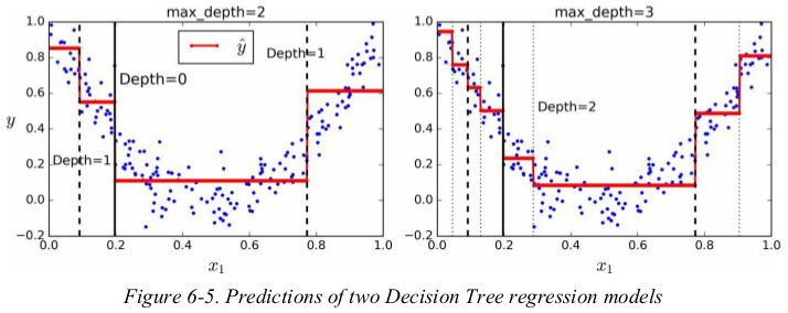
　　notice how the predicted value for each region is always the average target value of the instances in that region. the algorithm splits each region in a way that makes most training instances as close as possible to that predicted value. 

　　the CART algorithm works mostly the same way as earlier，except that instead of trying to split the training set in a way that minimizes impurity，it now tries to split the training set in a way that minimizes the MSE. 

　　Equation 6-4 shows the cost function that the algorithm tries to minimize: 

　　

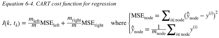
　　方程中的MSE就是平均数啊。

　　

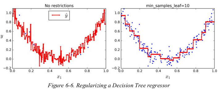
　　just like for classification tasks，Decision Trees are prone to overfitting when dealing with regression tasks. 

　　正则化的方法也与分类时相似

　　

Instability: 

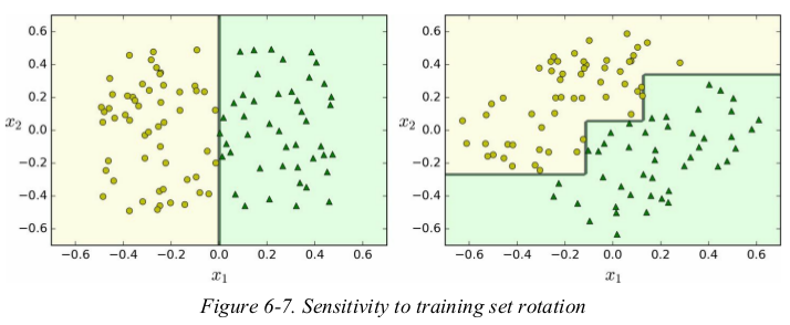
　　Decision Trees also have a few limitations. first，Decision Trees love orthogonal decision boundaries，which makes them sensitive to training set rotation.

　　for example，Figure 6-7 shows a simple linearly separable dataset: on the left，a Decision Tree can split it easily，while on the right，after the dataset is rotated by 45°，the decision boundary looks unnecessarily convoluted. although both Decision Trees fit the training set perfectly，it is very likely that the model on the right will not generalize well. one way to limit this problem is to use PCA，which often results in a better orientation of the training data. 

import numpy as np
import matplotlib.pyplot as plt
from matplotlib.colors import ListedColormap
from sklearn.tree import DecisionTreeClassifier

np.random.seed(6)
X = np.random.rand(100, 2) - 0.5
y = (X[:, 0] > 0).astype(np.float32) * 2

angle = np.pi / 4
rotation_matrix = np.array([[np.cos(angle), -np.sin(angle)], [np.sin(angle), np.cos(angle)]])
Xr = X.dot(rotation_matrix)

tree_clf1 = DecisionTreeClassifier(random_state=42)
tree_clf2 = DecisionTreeClassifier(random_state=42)
tree_clf1.fit(X, y)
tree_clf2.fit(Xr, y)


def plot_regression_predictions(tree_clf, X, y, axes=[-0.7, 0.7, -0.7, 0.7]):
    x1s = np.linspace(axes[0], axes[1], 100)
    x2s = np.linspace(axes[2], axes[3], 100)
    x1, x2 = np.meshgrid(x1s, x2s)
    X_new = np.c_[x1.ravel(), x2.ravel()]
    y_pred = tree_clf.predict(X_new).reshape(x1.shape)
    custom_cmap = ListedColormap(['#fafab0', '#9898ff', '#a0faa0'])
    plt.contourf(x1, x2, y_pred, alpha=0.3, cmap=custom_cmap)

    plt.plot(X[:, 0][y == 0], X[:, 1][y == 0], 'yo')
    plt.plot(X[:, 0][y == 2], X[:, 1][y == 2], 'g^')
    plt.axis(axes)
    plt.xlabel('$x_1$', fontsize=14)
    plt.ylabel('$x_2$', fontsize=14, rotation=0)


plt.figure(figsize=(11, 4))
plt.subplot(121)
plot_regression_predictions(tree_clf1, X, y)
plt.subplot(122)
plot_regression_predictions(tree_clf2, Xr, y)
plt.show()

　　

　　more generally，the main issue with Decision Trees is that they are very sensitive to small variations in the training data. for example，if you just remove the widest Iris-Versicolor from the iris training set(the one with petal 4.8 cm long and 1.8 cm wide) and train a new Decision Tree，you may get the model represented in Figure 6-8. as you can see，it looks very different from the previous Decision Tree (Figure 6-2). 

from sklearn.tree import DecisionTreeClassifier

iris = load_iris()
X = iris.data[:, 2:]  # petal length and width
y = iris.target

not_widest_versicolor = (X[:, 1] != 1.8) | (y == 2)
X_tweaked = X[not_widest_versicolor]
y_tweaked = y[not_widest_versicolor]

tree_clf = DecisionTreeClassifier(max_depth=2, random_state=40)
tree_clf.fit(X_tweaked, y_tweaked)


plt.figure(figsize=(8, 4))
plot_decision_boundary(tree_clf, X_tweaked, y_tweaked)
plt.plot([0, 7.5], [0.8, 0.8], "k-", linewidth=2)
plt.plot([0, 7.5], [1.75, 1.75], "k--", linewidth=2)
plt.text(1.0, 0.9, "Depth=0", fontsize=15)
plt.text(1.0, 1.80, "Depth=1", fontsize=13)
plt.show()

　　

　　

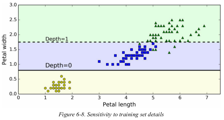
　　Random Forests can limit this instability by averaging predictions over many trees. 

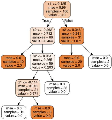
# 问题：画Figure 6-7时，错把分类图化成了回归图，但图本身并没有任何变化，由此发现了一个问题：对于同样的数据，同样的参数，只是使用的模型不同(DecisionTreeClassifier or DecisionTreeRegressor)时，划分树的thresholds是一样的，二者不同支出在于gini or mse、value的含义。

分类，

回归，

Exercises: 

1. What is the approximate depth of a Decision Tree trained (without restrictions) on a training set with 1 million instances?

　　one leaf per training instance if it is trained without restrictions.  log₂(10⁶) ≈ 20

2. Is a node’s Gini impurity generally lower or greater than itsparent’s? Is it generally lower/greater, or always lower/greater?

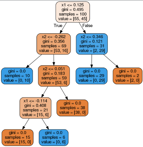
　　generally lower. however，if one child is smaller than the other，it is possible for it to have a higher Gini impurity than its parent，as long as this increase is more than compensated for by a decrease of the other child's impurity. for example，consider a node below: 

　　

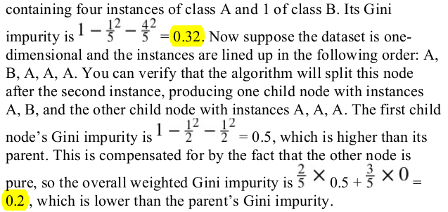
　　最后也是加权和

4. If a Decision Tree is underfitting the training set, is it a good idea to try scaling the input features?

　　Decision Trees don't care whether or not the training data is scaled or centered；that's one of the nice things about them. 

7. Train and fine-tune a Decision Tree for the moons dataset. 比较简单，训练也是瞬间完成。

from sklearn.datasets import make_moons
from sklearn.model_selection import train_test_split
from sklearn.tree import DecisionTreeClassifier
from sklearn.model_selection import GridSearchCV
from sklearn.metrics import accuracy_score

X, y = make_moons(n_samples=10000, noise=0.4, random_state=42)
X_train, X_test, y_train, y_test = train_test_split(X, y, test_size=0.2, random_state=42)

params = {'max_leaf_nodes': list(range(2, 100)), 'min_samples_split': [2, 3, 4]}

grid_search_cv = GridSearchCV(DecisionTreeClassifier(random_state=42), params, cv=3, verbose=1, n_jobs=-1)
grid_search_cv.fit(X_train, y_train)

y_pred = grid_search_cv.predict(X_test)
print(accuracy_score(y_test, y_pred))  # 0.8695

8. Grow a forest.

　　a. generate 1000 subsets of  the training set，each containing 100 instances selected randomly.

import numpy as np
from sklearn.datasets import make_moons
from sklearn.model_selection import train_test_split
from sklearn.tree import DecisionTreeClassifier
from sklearn.model_selection import GridSearchCV
from sklearn.metrics import accuracy_score
from sklearn.model_selection import ShuffleSplit
from sklearn.base import clone

n_trees = 1000
n_instances = 100
mini_sets = []

X, y = make_moons(n_samples=10000, noise=0.4, random_state=42)
X_train, X_test, y_train, y_test = train_test_split(X, y, test_size=0.2, random_state=42)

params = {'max_leaf_nodes': list(range(2, 100)), 'min_samples_split': [2, 3, 4]}

grid_search_cv = GridSearchCV(DecisionTreeClassifier(random_state=42), params, cv=3, verbose=1, n_jobs=-1)
grid_search_cv.fit(X_train, y_train)

# y_pred = grid_search_cv.predict(X_test)
# print(accuracy_score(y_test, y_pred))  # 0.8695


rs = ShuffleSplit(n_splits=n_trees, test_size=len(X_train) - n_instances, random_state=42)
for mini_train_index, mini_test_index in rs.split(X_train):  # 把8000切割为100、7900，切割1000次
    X_mini_train = X_train[mini_train_index]
    y_mini_train = y_train[mini_train_index]
    mini_sets.append((X_mini_train, y_mini_train))

forest = [clone(grid_search_cv.best_estimator_) for _ in range(n_trees)]

accuracy_scores = []

for tree, (X_mini_train, y_mini_train) in zip(forest, mini_sets):
    tree.fit(X_mini_train, y_mini_train)
    y_pred = tree.predict(X_test)
    accuracy_scores.append(accuracy_score(y_test, y_pred))

print(np.mean(accuracy_scores))  # 0.8054499999999999