Linear Regression
The Normal Equation
Computational Complexity
线性回归模型与MSE.


the normal equation:
a closed-form solution to find the value of θ that minimize the cost function.

generate some linear-looking data to test this equation. inv() to compute the inverse of a matrix,and dot() for matrix multiplication.
 1 np.random.seed(42)
 2 X = 2 * np.random.rand(100, 1)  # 怎么还有超过1的数值??
 3 y = 4 + 3 * X + np.random.randn(100, 1)
 4 # plt.plot(X, y, 'b.')
 5 # plt.xlabel('$x_1$', fontsize=18)  # '_': 下标,  '^': 上标
 6 # plt.ylabel('$y$', rotation=0, fontsize=18)  # 旋转角度, *rotation* may be 'horizontal', 'vertical', or a numeric value in degrees.
 7 # plt.axis([0, 2, 0, 15])
 8 # plt.show()
 9
10 X_b = np.c_[np.ones((100, 1)), X]  # add x0 = 1 to each instance, 求偏置项
11 theta_best = np.linalg.inv(X_b.T.dot(X_b)).dot(X_b.T).dot(y)
12 print(theta_best)
13 # [[4.21509616]
14 #  [2.77011339]]
15 #
16 X_new = np.array([[0], [2]])
17 X_new_b = np.c_[np.ones((2, 1)), X_new]
18 y_predict = X_new_b.dot(theta_best)
19 print(y_predict)  # [[4.21509616] [9.75532293]]
20 #
21 # plt.plot(X_new, y_predict, 'r-', linewidth=2, label='Predictions')  # label为图例
22 # plt.plot(X, y, 'b.')
23 # plt.xlabel("$x_1$", fontsize=18)
24 # plt.ylabel("$y$", rotation=0, fontsize=18)
25 # plt.legend(loc="upper left", fontsize=14)
26 # plt.axis([0, 2, 0, 15])
27 # plt.show()
28 #
29 lin_reg = LinearRegression()
30 lin_reg.fit(X, y)
31 print(lin_reg.intercept_, lin_reg.coef_)  # [4.21509616]; [[2.77011339]]
32 print(lin_reg.predict(X_new))  # [[4.21509616] [9.75532293]]
computational complexity:
the normal equation computes the inverse of XT· X,which is an n × n matrix(where n is the number of features). the computational complexity of inverting such a matrix is typically about O(n2.4) to O(n3) (depending on the implementation). the normal equation gets very slow when the number of features grows large.
on the positive side,this equation is linear with regards to the number of instances in the training set(O(m)),so it handles large training sets efficiently.
predictions are very fast: the computational complexity is linear with regards to both the number of instances you want to make predictions on and the number of features.
Gradient Descent
Batch Gradient Descent
Stochastic Gradient Descent
Mini-batch Gradient Descent
better suited for cases where there are a large number of features,or too many training instances to fit in memory.
the general idea of Gradient Descent is to tweak parameters iteratively in order to minimize a cost function.
it measures the local gradient of the error function with regards to the parameter vector θ,and it goes in the direction of descending gradient,once the gradient is zero,you have reached a minimum.
you start by filling θ with random values(this is called random initialization).
an important parameter in Gradient Descent is the size of the steps,determined by the learning rate hyperparameter. if the learning rate is too high,you might jump across the valley and end up on the other side,possibly even higher up than you were before. this might make the algorithm diverge,with larger and larger values,failing to find a good solution.
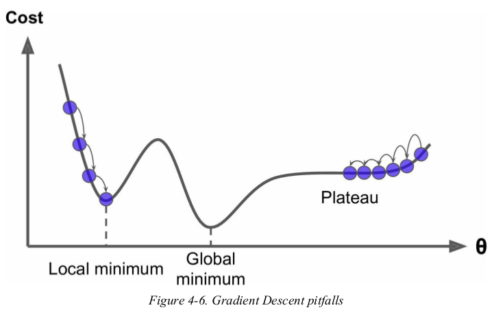
not all cost function look like nice regular bowls. there may be holes,ridges,plateaus,and all sorts of irregular terrains,making convergence to the minimum very difficult.
Figure4-6 shows the two main challenges with Gradient Descent: if the random initialization starts the algorithm on the left,then it will converge to a local minimum,which is not as good as the global minimum. if it starts on the right,then it will take a very long time to cross the plateau,and if you stop too early you will never reach the global minimum.
fortunately,the MSE cost function for a Linear Regression model happens to be a convex function,which means that if you pick any two points on the curve,the line segment joining them never crosses the curve. this implies that there are no local minima,just one global minimum. it is also a continuous function with a slope that never changes abruptly. these two facts have a great consequence: Gradient Descent is guaranteed to approach arbitrary close the global minimum(if you wait long enough and if the learning rate is not too high).
the cost function has the shape of a bowl,but it can be an elongated bowl if the features have very different scales. Figure4-7 shows Gradient Descent on a training set where feature 1 and 2 have the same scale(on the left),and on a training set where feature 1 has much smaller values than feature 2(on the right). 当然了,只有值较小跨度才会大呀。
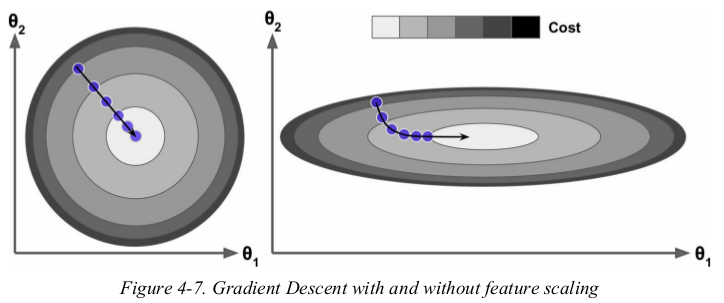
as you can see,on the left the Gradient Descent algorithm goes straight toward the minimum,thereby reaching it quickly,whereas on the right it first goes in a direction almost orthogonal to the direction of the global minimum,and it ends with a long march down an almost flat valley. it will eventually reach the minimum,but it will take a long time.
when using Gradient Descent,you should ensure that all features have a similar scale(e.g., using Scikit-Learn's StandardScaler class),or else it will take much longer to converge.
training a model means searching for a combination of model parameters that minimizes a cost function. it is a search in the model's parameter space: the more parameters a model has,the more dimensions this space has,and the harder the search is.
batch gradient descent:
to implement Gradient Descent,you need to compute the gradient of the cost function with regards to each model parameter θj. in other words,you need to calculate how much the cost function will change if you change θj just a little bit. this is called a partial derivative.
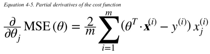
instead of computing these gradient individually,you can compute them all in one go. the gradient vector,noted ∇ θ MSE(θ),contains all the partial derivatives of the cost function(one for each model parameter).
Equation4-6 Gradient vector of the cost function,使用频率较高。
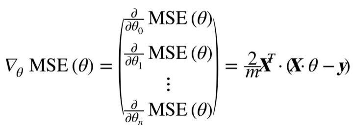
this formula involves calculations over the full training set X,at each Gradient Descent step. this is why the algorithm is called Batch Gradient Descent. as a result it is terribly slow on very large training set. however,Gradient Descent scales well with the number of features;training a Linear Regression model when there are hundreds of thousands of features is much faster using Gradient Descent than using the Normal Equation.
once you have the gradient vector,just subtract ∇θ MSE(θ) from θ,this is where the learning rate η comes into play.

 1 np.random.seed(42)
 2 X = 2 * np.random.rand(100, 1)  # 不是[0, 1)的均匀分布吗??大于1的数怎么也有??
 3 y = 4 + 3 * X + np.random.randn(100, 1)
 4
 5 X_b = np.c_[np.ones((100, 1)), X]
 6
 7 eta = 0.1
 8 n_iterations = 1000
 9 m = 100
10 np.random.seed(42)
11 theta = np.random.randn(2, 1)
12
13 for iteration in range(n_iterations):
14     gradients = 2/m * X_b.T.dot(X_b.dot(theta) - y)
15     theta = theta - eta * gradients
16 print(theta)  # [[4.21509616] [2.77011339]]
17
18 X_new = np.array([[0], [2]])
19 X_new_b = np.c_[np.ones((2, 1)), X_new]
20 print(X_new_b.dot(theta))  # [[4.21509616] [9.75532293]]
21
22
23 # 以不同学习率进行训练并作图
24 theta_path_bgd = []  # 这里没用到,是下面用的
25 def plot_gradient_descent(theta, eta, theta_path=None):
26     m = len(X_b)
27     plt.plot(X, y, 'b.')
28     n_iterations = 1000
29     for iteration in range(n_iterations):
30         if iteration < 10:
31             y_predict = X_new_b.dot(theta)
32             style = 'b-' if iteration > 0 else 'r--'
33             plt.plot(X_new, y_predict, style)
34         gradients = 2/m * X_b.T.dot(X_b.dot(theta) - y)
35         theta = theta - eta * gradients
36         if theta_path is not None:
37             theta_path.append(theta)
38     plt.xlabel('$x_1$', fontsize=18)
39     plt.axis([0, 2, 0, 15])  # 放在函数内,否则直线不与两边纵轴接触
40     plt.title(r'$eta = {}$'.format(eta), fontsize=16)  # 数学表达式,η
41
42 np.random.seed(42)
43 theta = np.random.randn(2, 1)
44 plt.figure(figsize=(10, 4))
45 plt.subplot(131)
46 plot_gradient_descent(theta, eta=0.02)
47 plt.ylabel('$y$', rotation=0, fontsize=18)
48 plt.subplot(132)
49 plot_gradient_descent(theta, eta=0.1, theta_path=theta_path_bgd)
50 plt.subplot(133)
51 plot_gradient_descent(theta, eta=0.5)
52 plt.show()
53 print(theta_path_bgd)

to find a good learning rate,you can use grid search. however,you may want to limit the number of iterations so that grid search can eliminate models that take too long to converge.
the approach to set the number of iterations: a simple solution is to set a very large number of iterations but to interrupt the algorithm when the gradient vector becomes tiny —— that is,when its norm becomes smaller than a tiny number called the tolerance —— because this happens when Gradient Descent has (almost) reached the minimum.
when the cost function is convex and its slope doesn't change abruptly,it can be shown that Batch Gradient Descent with a fixed learning rate has a convergence rate of O(1/ iterations). 即,if you divide the tolerance by 10,then the algorithm will have to run about 10 times more iterations.
stochastic gradient descent:
Batch Gradient Descent uses the whole training set to compute the gradient at every step,at the opposite extreme,Stochastic Gradient Descent just pick a random instance in the training set at every step and computed the gradients based only on that single instance. obviously this makes the algorithm much faster since it has very little data to manipulate at every iteration. it also makes it possible to train on huge training set,since only one instance needs to be in memory at each iteration.
on the other hand,due to its stochastic nature,this algorithm is much less regular than Batch Gradient Descent: instead of gently decreasing until it reaches the minimum,the cost function will bounce up and down,decreasing only on average. over time it will end up very close to the minimum,but once it gets there it will continue to bounce around,never settling down. so once the algorithm stops,the final parameter values are good,but not optimal.
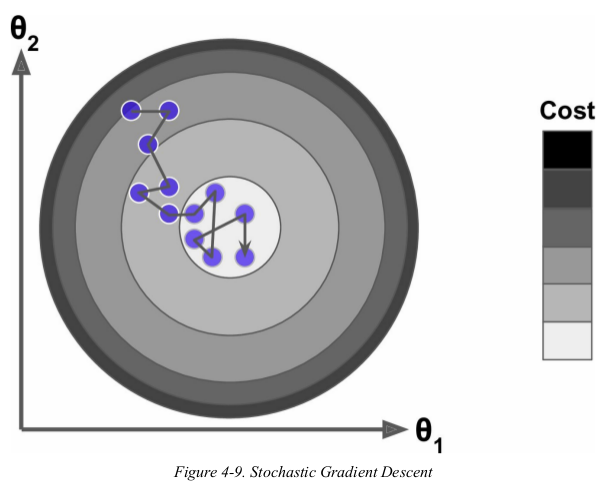
when the cost function is very irregular,如下图.
Stochastic Gradient Descent can help the algorithm jump out of local minima,so Stochastic Gradient Descent has a better chance of finding the global minimum than Batch Gradient Descent dose.
therefore randomness is good to escape from local optima,but bad because it means that the algorithm can never settle at the minimum. one solution to this dilemma is to gradually reduce the learning rate. the steps start out large(which helps make progress and escape local minima),then get smaller and smaller,allowing the algorithm to settle at the global minimum. this process is called simulated annealing,because it resembles the process of annealing in metallurgy where molten metal is slowly cooled down. the function that determines the learning rate at each iteration is called the learning schedule.
if the learning rate is reduced too quickly,you may get stuck in a local minimum,or even end up frozen halfway to the minimum. if the learning rate is reduced too slowly,you may jump around the minimum for a long time and end up with a suboptimal solution if you halt training too early. 这里要注意学习率降低快慢与学习率本身大小的区别。
 1 np.random.seed(42)
 2 X = 2 * np.random.rand(100, 1)  # 不是[0, 1)的均匀分布吗??大于1的数怎么也有??
 3 y = 4 + 3 * X + np.random.randn(100, 1)
 4
 5 X_b = np.c_[np.ones((100, 1)), X]
 6
 7 X_new = np.array([[0], [2]])
 8 X_new_b = np.c_[np.ones((2, 1)), X_new]
 9
10 m = len(X_b)
11 n_epochs = 50
12 t0, t1 = 5, 50
13
14
15 def learning_schedule(t):  # determines the learning rate at each iteration
16     return t0 / (t + t1)
17
18
19 np.random.seed(42)
20 theta = np.random.randn(2, 1)
21 for epoch in range(n_epochs):
22     for i in range(m):
23         if epoch == 0 and i < 20:
24             y_predict = X_new_b.dot(theta)
25             style = 'b-' if i > 0 else 'r--'
26             plt.plot(X_new, y_predict, style)
27
28         random_index = np.random.randint(m)  # 每次的输入都是随机的
29         xi = X_b[random_index: random_index+1]
30         yi = y[random_index: random_index+1]
31         gradients = 2 * xi.T.dot(xi.dot(theta) - yi)
32         eta = learning_schedule(epoch * m + i)
33         theta = theta - eta * gradients
34
35 print(theta)  # [[4.21076011] [2.74856079]]
36 plt.plot(X, y, 'b.')
37 plt.xlabel('$x_1$', fontsize=18)
38 plt.ylabel('$y$', rotation=0, fontsize=18)
39 plt.axis([0, 2, 0, 15])
40 plt.show()
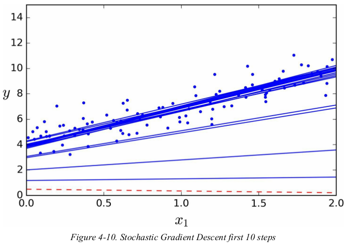
while the Batch Gradient Descent code iterated 1000 times through the whole training set,Stochastic Gradient Descent goes through the training set only 50times and reaches a fairly good solution.
since instances are picked randomly,some instances may be picked several times per epoch while others may not be picked at all. if you want to be sure that the algorithm goes through every instance at each epoch,another approach is to shuffle the training set,then go through it instance by instance,then shuffle it again,and so on. however,this generally converges more slowly.
to perform Linear Regression using SGD with Scikit-Learn,you can use the SGDRegressor class,which defaults to optimizing the squared error cost function. the following code runs 50 epochs,starting with a learning rate of 0.1,using the default learning schedule,and not use any regularization(penalty=None).
 1 from sklearn.linear_model import SGDRegressor
 2
 3 # max_iter: 注意是epochs, 不是iterations.
 4 # loss = 'squared_loss', optimize the squared error by default
 5 # penalty: 是否正则化
 6 # eta0: 初始学习率
 7 # learning_rate="invscaling", 是learning schedule
 8 #
 9 sgd_reg = SGDRegressor(max_iter=50, tol=-np.infty, penalty=None, eta0=0.1, random_state=42)
10 sgd_reg.fit(X, y.ravel())  # ravel把(100, 1)转为(100,)
11 print(sgd_reg.intercept_, sgd_reg.coef_)  # [4.16782089] [2.72603052]
mini-batch gradient descent:
Mini-batch GD computes the gradients on small random sets of instances called mini-batches.
the main advantage of Mini-batch GD over Stochastic GD is that you can get a performance boost from hardware optimization of matrix operations,especially when using GPUs.
the algorithm's progress in parameter space is less erratic than with SGD,especially with fairly large mini-batches. as a result,Mini-batch GD will end up walking around a bit closer to the minimum than SGD. on the other hand,it may be harder for it to escape from local minima.
Figure4-11 shows the paths taken by the three Gradient Descent algorithms in parameter space during training. they all end up near the minimum,but Batch GD's path actually stops at the minimum,while both Stochastic GD and Mini-batch GD continue to walk around.
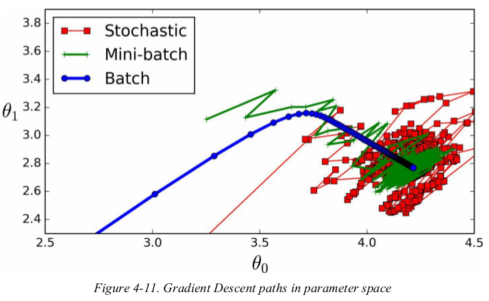
Stochastic GD and Mini-batch GD would also reach the minimum if you used a good learning rate.
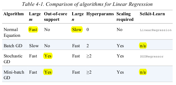
compare the algorithms for Linear Regression,recall that m is the number of training instances and n is the number of features.
Polynomial Regression
Surprisingly,you can actually use a linear model to fit nonlinear data. a simple way to do this is to add powers of each features as new features,then train a linear model on this extended set of features.
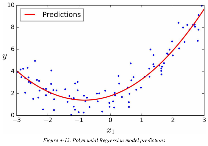
let's generate some nonlinear data,based on a simple quadratic equation. then use Scikit-Learn's PolynomialFeatures class to transform the training set,adding the square of each feature in the training set as new features.
 1 np.random.seed(42)
 2 m = 100
 3 X = 6 * np.random.rand(m, 1) - 3
 4 y = 0.5 * X ** 2 + X + 2 + np.random.randn(m, 1)
 5 # plt.plot(X, y, 'b.')
 6 # plt.xlabel("$x_1$", fontsize=18)
 7 # plt.ylabel("$y$", rotation=0, fontsize=18)
 8 # plt.axis([-3, 3, 0, 10])
 9 # plt.show()
10
11
12 from sklearn.preprocessing import PolynomialFeatures
13 from sklearn.linear_model import LinearRegression
14
15 poly_features = PolynomialFeatures(degree=2, include_bias=False)
16 X_poly = poly_features.fit_transform(X)
17 print(X[0])  # [-0.75275929]
18 print(X_poly[0])  # [-0.75275929  0.56664654]  算出一个平方数
19
20 lin_reg = LinearRegression()
21 lin_reg.fit(X_poly, y)
22 print(lin_reg.intercept_, lin_reg.coef_)  # [1.78134581] [[0.93366893 0.56456263]]  0.93为x的系数,0.56为x2的系数。
23
24
25 X_new = np.linspace(-3, 3, 100).reshape(100, 1)
26 X_new_poly = poly_features.transform(X_new)
27 y_new = lin_reg.predict(X_new_poly)
28 plt.plot(X, y, 'b.')
29 plt.plot(X_new, y_new, "r-", linewidth=2, label="Predictions")
30 plt.xlabel("$x_1$", fontsize=18)
31 plt.ylabel("$y$", rotation=0, fontsize=18)
32 plt.legend(loc="upper left", fontsize=14)
33 plt.axis([-3, 3, 0, 10])
34 plt.show()
note that when there are multiple features,Polynomial Regression is capable of finding relationships between features. this is made possible by the fact that PolynomialFeatures also adds all combinations of features up to the given degree. for example,if there were two features a and b,PolynomialFeatures with degree=3 would not only add the features a2,a3,b2 and b3,but also the combinations ab,a2b and ab2.
PolynomialFeatures(degree=3) transforms an array containing n features into an array containing (n + d) ! / d!×n! features. beware of the combinatorial explosion of the number of features.
Learning Curves
 1 from sklearn.preprocessing import StandardScaler
 2 from sklearn.pipeline import Pipeline
 3
 4 np.random.seed(42)
 5 m = 100
 6 X = 6 * np.random.rand(m, 1) - 3
 7 y = 0.5 * X ** 2 + X + 2 + np.random.randn(m, 1)
 8
 9 X_new = np.linspace(-3, 3, 100).reshape(100, 1)
10
11 for style, width, degree in (("g-", 1, 300), ("b--", 2, 2), ("r-+", 2, 1)):
12     polybig_features = PolynomialFeatures(degree=degree, include_bias=False)
13     std_scaler = StandardScaler()
14     lin_reg = LinearRegression()
15     polynomial_regression = Pipeline([
16             ("poly_features", polybig_features),
17             ("std_scaler", std_scaler),
18             ("lin_reg", lin_reg),
19         ])
20     polynomial_regression.fit(X, y)
21     y_newbig = polynomial_regression.predict(X_new)
22     plt.plot(X_new, y_newbig, style, label=str(degree), linewidth=width)
23
24 plt.plot(X, y, "b.", linewidth=3)
25 plt.legend(loc="upper left")
26 plt.xlabel("$x_1$", fontsize=18)
27 plt.ylabel("$y$", rotation=0, fontsize=18)
28 plt.axis([-3, 3, 0, 10])
29 plt.show()
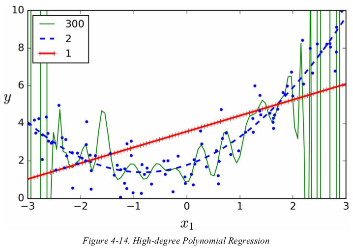
in general you won't know what function generated the data,so how can you decide how complex your model should be?how can you tell that your model is overfitting or underfitting the data?
another way is to look at the learning curves: these are plots of the model's performance on the training set and the validation set as a function of the training set size. to generate the plots,simply train the model several times on different sized subsets of the training set.
先看线性模型,
 1 import matplotlib.pyplot as plt
 2 import numpy as np
 3 from sklearn.metrics import mean_squared_error
 4 from sklearn.model_selection import train_test_split
 5 from sklearn.linear_model import LinearRegression
 6
 7
 8 def plot_learning_curves(model, X, y):
 9     X_train, X_val, y_train, y_val = train_test_split(X, y, test_size=0.2, random_state=10)
10     train_errors, val_errors = [], []
11     for m in range(1, len(X_train)):
12         model.fit(X_train[:m], y_train[:m])
13         y_train_predict = model.predict(X_train[:m])
14         y_val_predict = model.predict(X_val)
15         train_errors.append(mean_squared_error(y_train[:m], y_train_predict))
16         val_errors.append(mean_squared_error(y_val, y_val_predict))
17     plt.plot(np.sqrt(train_errors), 'r-+', linewidth=2, label='train')
18     plt.plot(np.sqrt(val_errors), 'b-', linewidth=3, label='val')
19     plt.legend(loc='upper right', fontsize=14)
20     plt.xlabel('Training set size', fontsize=14)
21     plt.ylabel('RMSE', fontsize=14)
22
23
24 np.random.seed(42)
25 m = 100
26 X = 6 * np.random.rand(m, 1) - 3
27 y = 0.5 * X ** 2 + X + 2 + np.random.randn(m, 1)
28
29 lin_reg = LinearRegression()
30 plot_learning_curves(lin_reg, X, y)
31 plt.axis([0, 80, 0, 3])
32 plt.show()
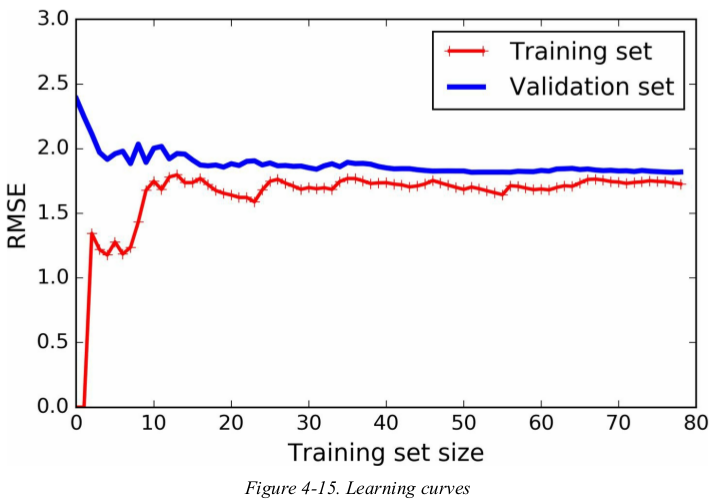
these learning curves are typically of an underfitting model. both curves have reaches a plateau;they are close and fairly high.
接下来看看the learning curves of a 10-degree polynomial model on the same data.
1 from sklearn.pipeline import Pipeline
2 from sklearn.preprocessing import PolynomialFeatures
3 polynomial_regression = Pipeline([
4     ('poly_features', PolynomialFeatures(degree=10, include_bias=False)),
5     ('lin_reg', LinearRegression()),
6 ])
7 plot_learning_curves(polynomial_regression, X, y)
8 plt.axis([0, 80, 0, 3])
9 plt.show()
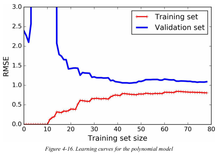
the error on the training data is much lower than with the Linear Regression model(Figure4-15).
there is a gap between the curves. this means that the model performs significantly better on the training data than on the validation data,which is the hallmark of an overfitting model. however,if you used a much larger training set,the two curves would continue to get closer.
the bias/ variance tradeoff:
a model's generalization error can be expressed as the sum of three very different errors:
Bias: this part of the generalization error is due to wrong assumptions,such as assuming that the data is linear when it is actually quadratic. a high-bias model is most likely to underfit the training data.
Variance: this part is due to the model's excessive sensitivity to small variations in the training data. a model with many degree of freedom is likely to have high variance,and thus to overfit the training data.
Irreducible error: this part is due to the noiseness of the data itself. the only way to reduce this part of the error is to clean up the data.
increasing a model's complexity will typically increase its variance and reduce its bias. conversely,reducing a model's complexity increases its bias and reduces its variance. this is a tradeoff.
Regularized Linear Models
the fewer degrees of freedom it has,the harder it will be for it to overfit the data. for example,a simple way to regularize a polynomial model is to reduce the number of polynomial degree. for a linear model,regularization is typically achieved by constraining the weights of the model.
three different ways to constrain the weights:
Ridge Regression、
Lasso Regression、
Elastic Net
Early Stopping
ridge regression:
Ridge Regression is a regularized version of Linear Regression: a regularization term equal to  is added to the cost function. this forces the learning algorithm to not only fit the data but also keep the model weights as small as possible.
ote that the regularization term should only be added to the cost function during training.
it is quite common for the cost function used during training to be different from the performance measure used for testing. apart from regularization,another reason why they might be different is that a good training cost function should have optimization-friendly derivatives,while the performance measure used for testing should be as close as possible to the final objective. a good example of is a classifier using a cost function such as the log loss but evaluated using precision/ recall.
the hyperparameter α control how much you want to regularize the model. if α=0 then Ridge Regression is just Linear Regression. if α is very large,then all weights end up very close to zero and the result is a flat line going through the data's mean.

note that the bias term θ0 is not regularized(the sum starts at i = 1, not 0). if we define W as the vector of feature weights(θ1 to θn),then the regularization term is simply equal to 1/2( // W //2 ),where // * //2 represents the l2 norm of the weight vector.
for Gradient Descent,just add aW to the MSE gradient vector(Equation4-6).
it is important to scale the data(e.g., using a StandardScaler) before performing Ridge Regression,as it is sensitive to the scale of the input features. this is true of most regularized models.
 1 import matplotlib.pyplot as plt
 2 import numpy as np
 3 from sklearn.pipeline import Pipeline
 4 from sklearn.preprocessing import PolynomialFeatures, StandardScaler
 5 from sklearn.linear_model import LinearRegression, Ridge
 6
 7 np.random.seed(42)
 8 m = 20
 9 X = 3 * np.random.rand(m, 1)
10 y = 1 + 0.5 * X + np.random.randn(m, 1) / 1.5
11 X_new = np.linspace(0, 3, 100).reshape(100, 1)
12
13
14 def plot_model(model_class, polynomial, alphas, **model_kargs):
15     for alpha, style in zip(alphas, ('b-', 'g--', 'r:')):  # 3个不同的α,三条线。
16         model = model_class(alpha, **model_kargs) if alpha > 0 else LinearRegression()  # α=0时,Ridge即LinearRegression。
17         if polynomial:
18             model = Pipeline([  # 扩展、缩放、训练
19                 ('poly_features', PolynomialFeatures(degree=10, include_bias=False)),
20                 ('std_scaler', StandardScaler()),
21                 ('regul_reg', model)
22             ])
23         model.fit(X, y)
24         y_new_regul = model.predict(X_new)
25         lw = 2 if alpha > 0 else 1
26         plt.plot(X_new, y_new_regul, style, linewidth=lw, label=r'$alpha = {}$'.format(alpha))
27         plt.plot(X, y, 'b.', linewidth=3)
28         plt.legend(loc='upper left', fontsize=15)
29         plt.xlabel('$x_1$', fontsize=18)
30         plt.axis([0, 3, 0, 4])
31
32
33 plt.figure(figsize=(8, 4))
34 plt.subplot(121)
35 plot_model(Ridge, polynomial=False, alphas=(0, 10, 100), random_state=42)
36 plt.ylabel('$y$', rotation=0, fontsize=18)
37 plt.subplot(122)
38 plot_model(Ridge, polynomial=True, alphas=(0, 10**-5, 1), random_state=42)
39 plt.show()
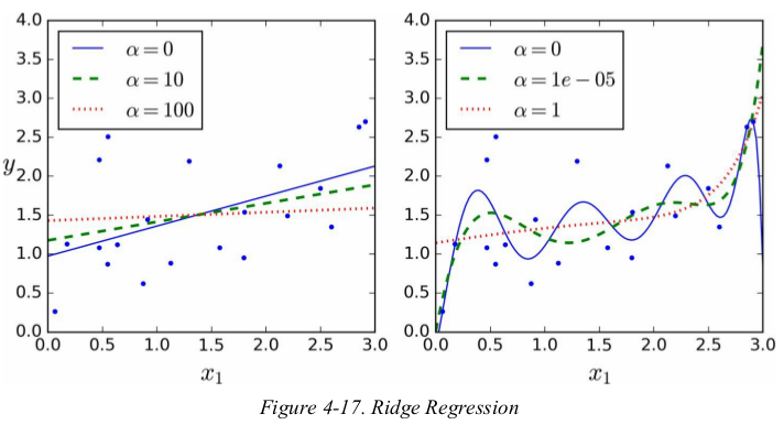
increasing α leads to flatter predictions(i.e., less extreme,more reasonable,少了极端值,多了一般值);this reduces the model's variance but increase its bias.
as with Linear Regression,we can perform Ridge Regression either by computing a closed-form equation or by performing Gradient Descent. the pros and cons are the same.

where A is the n × n identity matrix except with a 0 in the top-left cell,corresponding to the bias term.
perform Ridge Regression with Scikit-Learn using a closed-form solution(a variant of Equation4-9 using a matrix factorization technique by Andre-Louis Cholesky).
 1 from sklearn.linear_model import Ridge, SGDRegressor
 2
 3 np.random.seed(42)
 4 m = 20
 5 X = 3 * np.random.rand(m, 1)
 6 y = 1 + 0.5 * X + np.random.randn(m, 1) / 1.5
 7 X_new = np.linspace(0, 3, 100).reshape(100, 1)
 8
 9 ridge_reg = Ridge(alpha=1, solver='cholesky', random_state=42)
10 ridge_reg.fit(X, y)
11 print(ridge_reg.predict([[1.5]]))  # [[1.55071465]]
12
13 sgd_reg = SGDRegressor(max_iter=50, tol=-np.infty, penalty='l2', random_state=42)
14 sgd_reg.fit(X, y.ravel())
15 print(sgd_reg.predict([[1.5]]))  # [1.49838626]
the penalty hyperparameter sets the type of regularization term. specifying “l2” indicates that you want SGD to add a regularization term to the cost function equal to half the square of the l2 norm of the weight vector: this is simply Ridge Regression.
Lasso Regression:
Least Absolute Shrinkage and Selection Operator Regression(Lasso Regression) is another regularized version of Linear Regression: just like Ridge Regression,it adds a regularization term to the cost function,but it use the l1 norm of the weight vector instead of half the square of the l2 norm.

Figure4-18,与Figure4-17仅一点不同
 1 from sklearn.linear_model import Ridge, Lasso, SGDRegressor
 2
 3 np.random.seed(42)
 4 m = 20
 5 X = 3 * np.random.rand(m, 1)
 6 y = 1 + 0.5 * X + np.random.randn(m, 1) / 1.5
 7 X_new = np.linspace(0, 3, 100).reshape(100, 1)
 8
 9 plt.figure(figsize=(8, 4))
10 plt.subplot(121)
11 plot_model(Lasso, polynomial=False, alphas=(0, 0.1, 1), random_state=42)
12 plt.ylabel('$y$', rotation=0, fontsize=18)
13 plt.subplot(122)
14 plot_model(Lasso, polynomial=True, alphas=(0, 10**-7, 1), tol=1, random_state=42)
15 plt.show()

an important characteristic of Lasso Regression is that it tends to completely eliminate the weights of the least important features(i.e., set them to zero). for example,the dashed line in the right plot on Figure4-18(with α = 10-7 ) looks quadratic,almost linear: all the weights for the high-degree polynomial features are equal to zero.
下面是Lasso 和 Ridge 的对比图:
 1 import matplotlib.pyplot as plt
 2 import numpy as np
 3
 4 t1a, t1b, t2a, t2b = -1, 3, -1.5, 1.5
 5
 6 # ignoring bias term
 7 t1s = np.linspace(t1a, t1b, 500)
 8 t2s = np.linspace(t2a, t2b, 500)
 9 t1, t2 = np.meshgrid(t1s, t2s)
10 T = np.c_[t1.ravel(), t2.ravel()]
11 Xr = np.array([[-1, 1], [-0.3, -1], [1, 0.1]])
12 yr = 2 * Xr[:, :1] + 0.5 * Xr[:, 1:]
13 # ` - yr.T`确定椭圆中心的位置;`**2`平方确定为椭圆,而不是直线
14 J = (1/len(Xr) * np.sum((T.dot(Xr.T) - yr.T)**2, axis=1)).reshape(t1.shape)
15
16 N1 = np.linalg.norm(T, ord=1, axis=1).reshape(t1.shape)
17 N2 = np.linalg.norm(T, ord=2, axis=1).reshape(t1.shape)
18
19 t_min_idx = np.unravel_index(np.argmin(J), J.shape)  # (333, 374)
20 t1_min, t2_min = t1[t_min_idx], t2[t_min_idx]
21
22 t_init = np.array([[0.25], [-1]])
23
24
25 def bgd_path(theta, X, y, l1, l2, core=1, eta=0.1, n_iterations=50):
26     path = [theta]
27     for iteration in range(n_iterations):
28         gradients = core * 2 / len(X) * X.T.dot(X.dot(theta) - y) + l1 * np.sign(theta) + 2 * l2 * theta
29
30         theta = theta - eta * gradients
31         path.append(theta)
32     return np.array(path)
33
34
35 plt.figure(figsize=(12, 8))
36 for i, N, l1, l2, title in ((0, N1, 0.5, 0, "Lasso"), (1, N2, 0, 0.1, "Ridge")):
37     JR = J + l1 * N1 + l2 * N2 ** 2
38
39     tr_min_idx = np.unravel_index(np.argmin(JR), JR.shape)
40     t1r_min, t2r_min = t1[tr_min_idx], t2[tr_min_idx]
41
42     levelsJ = (np.exp(np.linspace(0, 1, 20)) - 1) * (np.max(J) - np.min(J)) + np.min(J)
43     levelsJR = (np.exp(np.linspace(0, 1, 20)) - 1) * (np.max(JR) - np.min(JR)) + np.min(JR)
44     levelsN = np.linspace(0, np.max(N), 10)
45
46     path_J = bgd_path(t_init, Xr, yr, l1=0, l2=0)
47     path_JR = bgd_path(t_init, Xr, yr, l1, l2)
48     path_N = bgd_path(t_init, Xr, yr, np.sign(l1) / 3, np.sign(l2), core=0)
49
50     plt.subplot(221 + i * 2)
51     plt.grid(True)
52     plt.axhline(y=0, color='k')
53     plt.axvline(x=0, color='k')
54     plt.contourf(t1, t2, J, levels=levelsJ, alpha=0.9)
55     plt.contour(t1, t2, N, levels=levelsN)
56     plt.plot(path_J[:, 0], path_J[:, 1], "w-o")
57     plt.plot(path_N[:, 0], path_N[:, 1], "y-^")
58     plt.plot(t1_min, t2_min, "rs")
59     plt.title(r"$ell_{}$ penalty".format(i + 1), fontsize=16)
60     plt.axis([t1a, t1b, t2a, t2b])
61     if i == 1:
62         plt.xlabel(r"$	heta_1$", fontsize=20)
63     plt.ylabel(r"$	heta_2$", fontsize=20, rotation=0)
64
65     plt.subplot(222 + i * 2)
66     plt.grid(True)
67     plt.axhline(y=0, color='k')
68     plt.axvline(x=0, color='k')
69     plt.contourf(t1, t2, JR, levels=levelsJR, alpha=0.9)
70     plt.plot(path_JR[:, 0], path_JR[:, 1], "w-o")
71     plt.plot(t1r_min, t2r_min, "rs")
72     plt.title(title, fontsize=16)
73     plt.axis([t1a, t1b, t2a, t2b])
74     if i == 1:
75         plt.xlabel(r"$	heta_1$", fontsize=20)
76
77 plt.show()
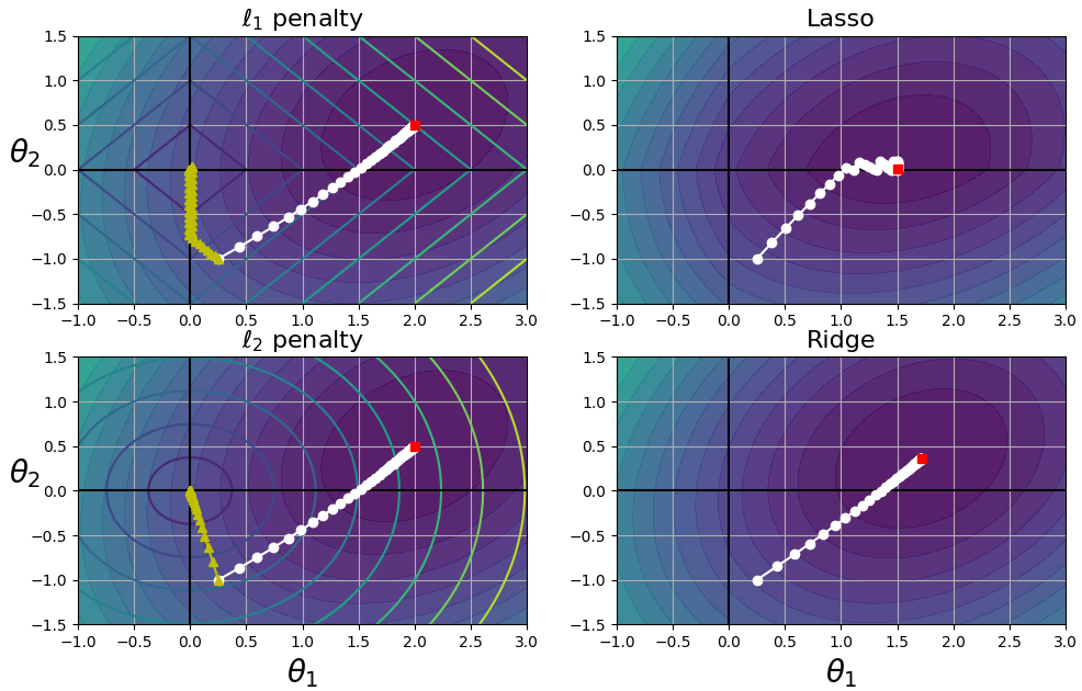
左上图,椭圆轮廓表示没有正则化时(α = 0)的MSE损失函数,白色圆点表示该损失函数的BGD过程;菱形轮廓表示只有正则化时(α → ∞)的 l1 penalty,绿色三角形表示该 penalty 的BGD过程。notice how the path first reaches θ1 = 0,then rolls down a gutter until it reaches θ2 = 0. 右上图,轮廓表示相同的损失函数加上一个 α = 0.5 的 l1 penalty,the global minimum is on the θ2 = 0 axis. BGD first reaches θ2 = 0,then rolls down the gutter until it reaches the global minimum. the two bottom plots show the l2 penalty instead. the regularized minimum is closer to θ = 0 than the unregularized minimum,but the weights don't get fully eliminated.
on the Lasso cost function,the BGD path tends to bounce across the gutter toward the end. this is because the slope changes abruptly at θ2 = 0. you need to gradually reduce the learning rate in order to actually converge to the global minimum.
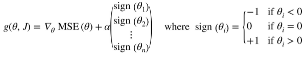
the Lasso cost function is not differentiable at θi = 0(for i = 1, 2, ..., n),but Gradient Descent still works fine if you use a subgradient vector g instead when any θi = 0.
Equation4-11 Lasso Regression subgradient vector
 1 import numpy as np
 2 from sklearn.linear_model import Lasso, SGDRegressor
 3
 4 np.random.seed(42)
 5 m = 20
 6 X = 3 * np.random.rand(m, 1)
 7 y = 1 + 0.5 * X + np.random.randn(m, 1) / 1.5
 8 X_new = np.linspace(0, 3, 100).reshape(100, 1)
 9
10 lasso_reg = Lasso(alpha=0.1, random_state=42)
11 lasso_reg.fit(X, y)
12 print(lasso_reg.predict([[1.5]]))  # [1.53788174]
13
14 sgd_reg = SGDRegressor(max_iter=50, tol=-np.infty, penalty='l1', alpha=0.1, random_state=42)
15 sgd_reg.fit(X, y.ravel())
16 print(sgd_reg.predict([[1.5]]))  # [1.46612563]
Elastic Net:
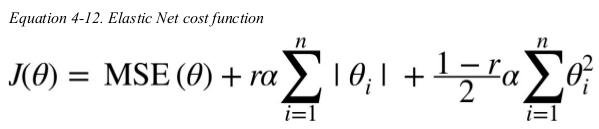
Elastic Net is a middle ground between Ridge Regression and Lasso Regression. the regularization term is a simple mix of both Ridge and Lasso's regularization terms,and you can control the mix ratio r. when r = 0,Elastic Net is equivalent to Ridge Regression,and when r = 1,it is equivalent to Lasso Regression.
 1 import numpy as np
 2 from sklearn.linear_model import ElasticNet
 3
 4 np.random.seed(42)
 5 m = 20
 6 X = 3 * np.random.rand(m, 1)
 7 y = 1 + 0.5 * X + np.random.randn(m, 1) / 1.5
 8 X_new = np.linspace(0, 3, 100).reshape(100, 1)
 9
10 elastic_net = ElasticNet(alpha=0.1, l1_ratio=0.5, random_state=42)
11 elastic_net.fit(X, y)
12 print(elastic_net.predict([[1.5]]))  # [1.54333232]
so when should you use Linear Regression,Ridge,Lasso,or Elastic Net?it is almost always preferable to have at least a little bit of regularization,so generally you should avoid plain Linear Regression. Ridge is a good default,but if you suspect that only a few features are actually useful,you should prefer Lasso or Elastic Net since they tend to reduce the useless features' weights down to zero as we have discussed. in general,Elastic Net is preferred over Lasso since Lasso may behave erratically when the number of features is greater than the number of training instances or when several features are strongly correlated.
Early Stopping:
a very different way to regularize iterative learning algorithms such as Gradient Descent is to stop training as soon as the validation error reaches a minimum. this is called early stopping.
 1 import numpy as np
 2 import matplotlib.pyplot as plt
 3 from sklearn.model_selection import train_test_split
 4 from sklearn.pipeline import Pipeline
 5 from sklearn.preprocessing import PolynomialFeatures, StandardScaler
 6 from sklearn.linear_model import SGDRegressor
 7 from sklearn.metrics import mean_squared_error
 8 from sklearn.base import clone
 9
10 np.random.seed(42)
11 m = 100
12 X = 6 * np.random.rand(m, 1) - 3
13 y = 2 + X + 0.5 * X ** 2 + np.random.randn(m, 1)
14
15 X_train, X_val, y_train, y_val = train_test_split(X[:50], y[:50].ravel(), test_size=0.5, random_state=10)
16
17 poly_scaler = Pipeline([
18     ('poly_features', PolynomialFeatures(degree=90, include_bias=False)),
19     ('std_scaler', StandardScaler()),
20 ])
21 X_train_poly_scaled = poly_scaler.fit_transform(X_train)
22 X_val_poly_scaled = poly_scaler.transform(X_val)
23
24 # when the fit() method is called, it just continues training where it left off instead of restarting from scratch.
25 sgd_reg = SGDRegressor(max_iter=1,
26                        tol=-np.infty,
27                        penalty=None,
28                        eta0=0.0005,
29                        warm_start=True,
30                        learning_rate='constant',
31                        random_state=42)
32 n_epochs = 500
33 minimum_val_error = float('inf')
34 best_epoch = None
35 best_model = None
36 train_errors, val_errors = [], []
37
38 for epoch in range(n_epochs):  # epoch为x轴
39     sgd_reg.fit(X_train_poly_scaled, y_train)
40     y_train_predict = sgd_reg.predict(X_train_poly_scaled)
41     y_val_predict = sgd_reg.predict(X_val_poly_scaled)
42     val_error = mean_squared_error(y_val, y_val_predict)
43     train_errors.append(mean_squared_error(y_train, y_train_predict))
44     val_errors.append(val_error)
45     if val_error < minimum_val_error:  # 保存最优模型的参数
46         minimum_val_error = val_error
47         best_epoch = epoch
48         best_model = clone(sgd_reg)
49
50 best_val_rmse = np.sqrt(val_errors[best_epoch])
51 best_val_rmse -= 0.03  # 为何??
52 plt.plot([0, n_epochs], [best_val_rmse, best_val_rmse], 'k:', linewidth=2)  # 一条水平线
53 plt.plot(np.sqrt(train_errors), 'r--', linewidth=2, label='Training set')  # If not given, they default to [0, ..., N-1].--from doc.
54 plt.plot(np.sqrt(val_errors), 'b-', linewidth=3, label='Validation set')
55 plt.legend(loc='upper right', fontsize=14)
56 plt.xlabel('Epoch', fontsize=14)
57 plt.ylabel('RMSE', fontsize=14)
58 plt.annotate('Best model',
59              xy=(best_epoch, best_val_rmse),
60              xytext=(best_epoch, best_val_rmse+1),
61              ha='center',  # 文档中没涉及,注释文字相对箭头的位置
62              arrowprops=dict(facecolor='black', shrink=0.05),  # Fraction of total length to shrink from both ends, 从两端收缩的总长度的百分比
63              fontsize=16,  # Additional kwargs are passed to Text.
64              )
65 plt.show()
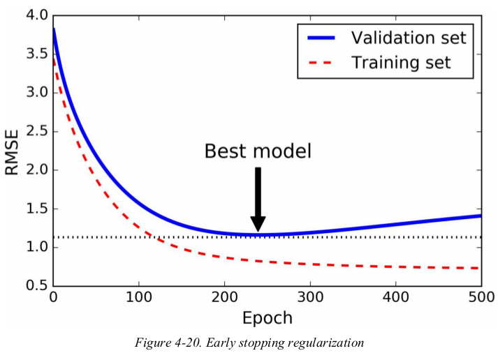
Figure4-20 shows a complex model being trained using Batch Gradient Descent. as the epochs go by,the algorithm learns and its prediction error (RMSE) on the training set naturally goes down,and so does its prediction error on the validation set. however,after a while the validation error stops decreasing and actually starts to go back up. this indicates that the model has started to overfit the training data. with early stopping you just stop training as soon as the validation error reaches the minimum. it is such a simple and efficient regularization technique.
with Stochastic and Mini-batch Gradient Descent,the curves are not so smooth,and it may be hard to know whether you have reached the minimum or not. One solution is to stop only after the validation error has been above the minimum for some time,then roll back the model parameters to the points where the validation error was at a minimum.
Logistics Regression
Estimating Probabilities
Training and Cost Function
Decision Boundaries
Softmax Regression
as we discussed before,some regression algorithms can be used for classification as well (and vice versa). Logistic Regression(also called Logit Regression) is commonly used to estimate the probability that an instance belongs to a particular class. if the estimate probability is greater than 50%,then the model predicts that the instance belongs to that class,or else it predicts that it does not,this makes it a binary classifier.
Estimating Probabilities:
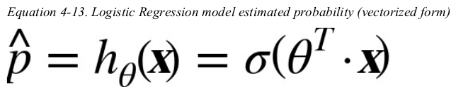
just like a Linear Regression model,a Logistics Regression model computes a weights sum of the input features(plus a bias term),but instead of outputting the result directly like the Linear Regression model does,it outputs the logistic of this result.
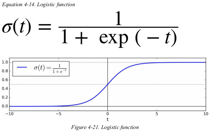
the logistic —— also called the logit,noted σ(·) —— is a sigmoid function(i.e., S-shaped) that outputs a number between 0 and 1.
once the Logistics Regression model has estimated the probability ![]() that an instance x belongs to the positive class,it can make its prediction y' easily.
that an instance x belongs to the positive class,it can make its prediction y' easily.

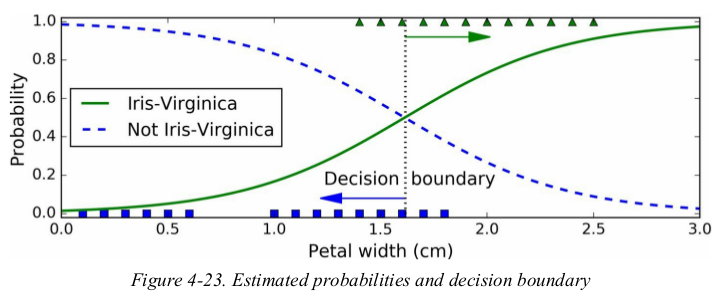
Notice that σ(t) < 0.5 when t < 0,and σ(t) ≥ 0.5 when t ≥ 0,so a Logistic Regression model predicts 1 if θT · x is positive,and 0 if it is negative.
Training and Cost Function:
the objective of training is to set the parameter vector θ so that the model estimates high probabilities for positive instances(y = 1) and low probabilities for negative instances(y = 0).
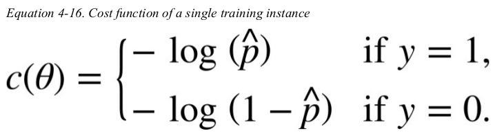
this cost function makes sense because -log(t) grows very large when t approaches 0,so the cost will be large if the model estimates a probability close to 0 for a positive instance,and it will also be very large if the model estimates a probability close to 1 for a negative instance.
on the other hand,-log(t) is close to 0 when t is close to 1,so the cost will be close to 0 if the estimated probability is close to 1 for a positive instance or close to 0 for a negative instance. this is precisely what we want.
the cost function over the whole training set is simply the average cost over all training instances. it can be written in a single expression,called the log loss.
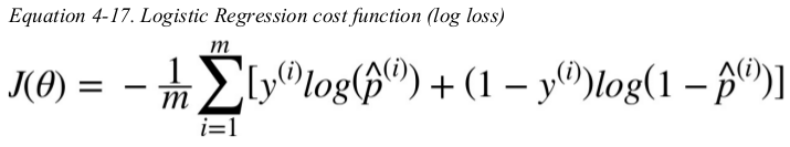
the bad news is that there is no known closed-form equation to compute the value of θ that minimizes this cost function. the good news is that this cost function is convex,so Gradient Descent(or any other optimization algorithm) is guaranteed to find the global minimum(if the learning rate is not too large and you wait long enough). the partial derivatives of the function with regards to the jth model parameter θj is given below.
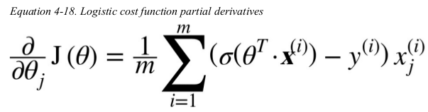
this equation looks very much like Equation4-5,for each instance it computes the prediction error and multiplies it by the jth feature value,and then it computes the average over all training instances. once you have the gradient vector containing all the partial derivatives you can use it in the Batch Gradient Descent algorithm.
That’s it: you now know how to train a Logistic Regression model. For Stochastic GD you would of course just take one instance at a time,and for Mini-batch GD you would use a mini-batch at a time.
Decision Boundaries:
用一个特征(petal width)判断是否是Iris-Virginia,决策边界为一个数值(1.61561562). predict输出类别,predict_proba输出各类别概率.
 1 from sklearn.linear_model import LogisticRegression
 2
 3 iris = datasets.load_iris()
 4 X = iris['data'][:, 3:]  # one feature: petal width
 5 y = (iris['target'] == 2).astype(np.int)
 6
 7 log_reg = LogisticRegression(solver="liblinear", random_state=42)
 8 log_reg.fit(X, y)
 9
10 X_new = np.linspace(0, 3, 1000).reshape(-1, 1)
11 y_proba = log_reg.predict_proba(X_new)  # Probability estimates  # binary classifier (1000, 2)  # X_new、y_proba都已按序排列,便于求决策边界。
12 decision_boundary = X_new[y_proba[:, 1] >= 0.5][0]  # [1.61561562]  # 数组是从大到小排列的  # 概率大于0.5的决策边界,这个`0.5`是固定的,模型本身就是这么来判断的
13
14 plt.figure(figsize=(8, 3))
15 plt.plot(X[y == 0], y[y == 0], 'bs')  # 负例
16 plt.plot(X[y == 1], y[y == 1], 'g^')  # 正例
17 plt.plot([decision_boundary, decision_boundary], [-1, 2], 'k:', linewidth=2)  # 竖线
18 plt.plot(X_new, y_proba[:, 1], 'g-', linewidth=2, label='Iris-Virginica')       # 正例
19 plt.plot(X_new, y_proba[:, 0], 'b--', linewidth=2, label='Not Iris-Virginica')  # 反例
20 plt.text(decision_boundary+0.02, 0.15, 'Decision boundary', fontsize=14, color='k', ha='center')
21 plt.arrow(decision_boundary, 0.08, -0.3, 0, head_width=0.05, head_length=0.1, fc='b', ec='b')  # 前两个参数表示the arrow base,即箭头起点;第3、4个参数(dx、dy)表示在x、y方向上的长度。fc和ec分别为facecolor和edgecolor的简写。
22 plt.arrow(decision_boundary, 0.92, 0.3, 0, head_width=0.05, head_length=0.1, fc='g', ec='g')
23 plt.xlabel("Petal width (cm)", fontsize=14)
24 plt.ylabel("Probability", fontsize=14)
25 plt.legend(loc="center left", fontsize=14)
26 plt.axis([0, 3, -0.02, 1.02])
27 plt.show()
1 print(log_reg.predict([[1.7], [1.5]]))  # [1 0]
2 print(log_reg.predict_proba([[1.7], [1.5]]))
3
4 # [[0.44316529 0.55683471]
5 #  [0.57328164 0.42671836]]
用两个特征(patal width and length)判断是否是Iris-Virginia.
 1 from sklearn.linear_model import LogisticRegression
 2
 3 iris = datasets.load_iris()
 4 X = iris['data'][:, (2, 3)]
 5 y = (iris['target'] == 2).astype(np.int)
 6
 7 log_reg = LogisticRegression(solver="liblinear", C=10**10, random_state=42)  # C=10**10, control the regularization strength
 8 log_reg.fit(X, y)
 9 x0, x1 = np.meshgrid(  # x0、x1的shape都为(200, 500)
10  # reshape: (500,) --> (500, 1)
11     np.linspace(2.9, 7, 500).reshape(-1, 1),
12     np.linspace(0.8, 2.7, 200).reshape(-1, 1),
13 )
14 X_new = np.c_[x0.ravel(), x1.ravel()]  # (100000, 2)
15 y_proba = log_reg.predict_proba(X_new)  # Probability estimates  # (100000, 2)
16
17 plt.figure(figsize=(10, 4))
18 plt.plot(X[y == 0, 0], X[y == 0, 1], 'bs')  # 负例
19 plt.plot(X[y == 1, 0], X[y == 1, 1], 'g^')  # 正例
20 from matplotlib.colors import ListedColormap
21 custom_cmap = ListedColormap(['#fafab0', '#9898ff', '#a0faa0'])  # 自定制颜色
22 plt.contourf(x0, x1, log_reg.predict(X_new).reshape(x0.shape), cmap=custom_cmap)
23 zz = y_proba[:, 1].reshape(x0.shape)
24 contour = plt.contour(x0, x1, zz, cmap=plt.cm.brg)  # 几条概率线
25 left_right = np.array([2.9, 7])
26 print(log_reg.coef_, log_reg.intercept_)  # [[ 5.75286199 10.44454566]] [-45.26057652]
27 boundary = -(log_reg.coef_[0][0] * left_right + log_reg.intercept_[0]) / log_reg.coef_[0][1]  # 怎么来的呢??
28 print(boundary)  # [2.73609573 0.47781328]
29 plt.clabel(contour, inline=1, fontsize=12)  # 概率线上的概率值
30 plt.plot(left_right, boundary, 'k--', linewidth=3)  # 过两个坐标做一条直线,注意坐标轴一般都不是0轴,卡了我好长时间,一直感觉有问题,就是找不到问题出在哪
31 plt.text(3.5, 1.5, "Not Iris-Virginica", fontsize=14, color="b", ha="center")
32 plt.text(6.5, 2.3, "Iris-Virginica", fontsize=14, color="g", ha="center")
33 plt.xlabel("Petal length", fontsize=14)
34 plt.ylabel("Petal width", fontsize=14)
35 plt.axis([2.9, 7, 0.8, 2.7])
36 plt.show()

the dashed line represents the points where the model estimates a 50% probability: this is the linear boundary. each parallel line represents the points where the model outputs a specific probability,from 15% to 90%. all the flowers beyond the top-right line have an over 90% chance of being Iris-Virginia according to the model.
just like the other linear models,Logistic Regression models can be regularized using l1 or l2 penalties. Scikit-Learn actually adds an l2 penalty by default.
the hyperparameter controlling the regularization strength of a Scikit-Learn LogisticRegression model is not alpha,but its inverse: C. the higher the value of C,the less the model is regularized.
Softmax Regression:
the Logistic Regression model can be generalized to support multiple classes directly,without having to train and combine multiple binary classifiers. this is called Softmax Regression,or Multinomial Logistic Regression.
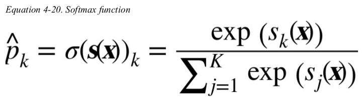
main idea: when given an instance x,the Softmax Regression model first computes a score sk(x) for each class k,then estimates the probability of each class by applying the softmax function(also called the normalized exponential) to the scores.
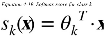
the equation to compute sk(x) is just like the equation for Linear Regression prediction.
once you have computed the score of every class for the instance x,you can estimate the probability that the instance belongs to class k by running the scores through the softmax function: it computes the exponential of every score,then normalizes them(dividing by the sum of all the exponentials).
just like the Logistic Regression classifier,the Softmax Regression classifier predicts the class with the highest estimated probability (which is simply the class with the highest score). 单调递增。
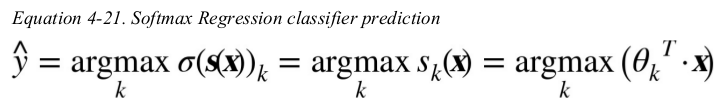
the argmax operator returns the value of a variable that maximizes a function. in this equation,it returns the value of k that maximizes the estimated probability  .
.
Note: the Softmax Regression classifier predicts only one class at a time(i.e., it is multiclass,not multi output) so it should be used only with mutually exclusive classes such as different types of plants. you cannot use it to recognize multiple people in one picture.
the objective of training is to have a model that estimates a high probability for the target class(and consequently a low probability for the other classes). minimizing the cost function shown in Equation4-22,called the cross entropy,should lead to this objective because it penalties the model when it estimates a low probability for a target class.
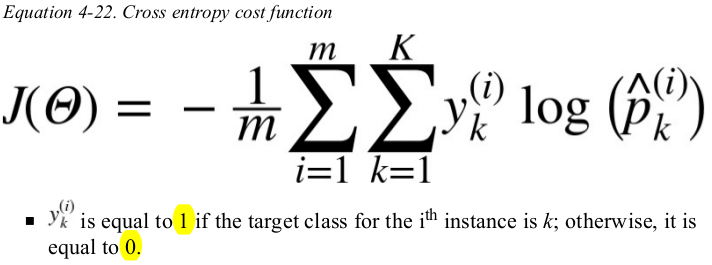
notice that when there are just two classes(K=2),this cost function is equivalent to the Logistic Regression's cost function.
the gradient vector of this cost function with regards to θk is given by Equation4-23:
Equation 4-23. Cross entropy gradient vector for class k
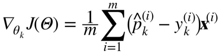
now you can compute the gradient vector for every class,then use Gradient Descent(or any other optimization algorithm) to find the parameter matrix that minimizes the cost function.
Let's use Softmax Regression to classify the iris flowers into all three classes. Scikit-Learn's LogisticRegression uses one-versus-all by default when you train it on more than two classes,but you can set multi_class hyperparameter to “multinomial” to switch it to Softmax Regression instead. you must also specify a solver that supports Softmax Regression,such as the “lbfgs” solver. it also applies l2 regularization by default,which you can control using the hyperparameter C.
 1 from sklearn.linear_model import LogisticRegression
 2
 3 iris = datasets.load_iris()
 4 X = iris['data'][:, (2, 3)]
 5 y = iris['target']
 6
 7 softmax_reg = LogisticRegression(C=10, solver='lbfgs', multi_class='multinomial')
 8 softmax_reg.fit(X, y)
 9
10 print(softmax_reg.predict([[5, 2]]))  # [2]
11 print(softmax_reg.predict_proba([[5, 2]]))  # [[6.38014896e-07 5.74929995e-02 9.42506362e-01]]
最后一个图。。
Exercises:
5. Suppose you use Batch Gradient Descent and you plot the validation error at every epoch. If you notice that the validation error consistently goes up, what is likely going on? How can you fix this?
if the validation error consistently goes up after every epoch,then one probability is that the leaning rate is too high and the algorithm is diverging. if the training error also goes up,then this is clearly the problem and you should reduce the learning rate. however,if the training error is not going up,then your model is overfitting the training set and you should stop training.
11. Suppose you want to classify pictures as outdoor/indoor and daytime/nighttime. Should you implement two Logistic Regression classifiers or one Softmax Regression classifier?
if you want to classify pictures as outdoor/ indoor and daytime/ nighttime,since these are not exclusive classes(i.e., all four combination are possible) you should train two Logistic Regression classifiers.