壁虎书2 End-to-End Machine Learning Project

the main steps: 

　　1. look at the big picture

　　2. get the data

　　3. discover and visualize the data to gain insights

　　4. prepare the data for machine learning algorithms

　　5. select a model and train it

　　6. fine-tune your model

　　7. present your solution

　　8. launch，monitor，and maintain your system

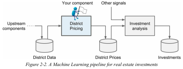
a sequence of processing component is called a data pipeline. 

components typically run asynchronously.

Look at the Big Picture

　　Frame the Problem

　　Select a Performance Measure

　　Check the Assumption

frame the problem:

　　is it supervised，unsupervised，or reinforcement learning? 

　　is it a classification task，a regression task，or something else?

　　batch learning or online learning techniques?

　　

select a performance measure:

　　a typical performance measure for regression problems is the Root Mean Square Error(RMSE). it measures the standard deviation of the errors the system makes in its predictions. 

　　

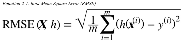
　　even though the RMSE is generally the preferred performance measure for regression tasks，in some contexts you may prefer to use another function: Mean ABsolute Error(Average Absolute Deviation).

　　

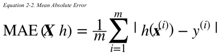
　　computing the root of a sum of squares(RMSE) corresponds to the Euclidian norm, computing the sum of absolutes(MAE) corresponds to the Manhattan norm. so the higher the norm index，the more it focuses on large values and neglects small ones. this is why the RMSE is more sensitive to outliers than the MAE.

Get the Data

　　Create the Workspace

　　Download the Data

　　Take a Quick Look at the Data Structure

　　Create a Test Set

download the data: 

　　in typical environments your data would be available in a relational database(or some other common database) and spread across multiple tables/ documents/ files. To access it, you would first need to get your credentials and access authorizations，and familiarize yourself with the data schema.

　　下载并提取数据

import os
from six.moves import urllib
import tarfile  # 标准库


DOWNLOAD_ROOT = 'https://raw.githubusercontent.com/ageron/handson-ml/master/'
HOUSING_PATH = 'datasets/housing'
HOUSING_URL = DOWNLOAD_ROOT + HOUSING_PATH + '/housing.tgz'


def fetch_housing_data(housing_url=HOUSING_URL, housing_path=HOUSING_PATH):
    if not os.path.isdir(housing_path):
        os.makedirs(housing_path)
    tgz_path = os.path.join(housing_path, 'housing.tgz')
    urllib.request.urlretrieve(housing_url, tgz_path)  # 下载文件
    housing_tgz = tarfile.open(tgz_path)
    housing_tgz.extractall(path=housing_path)  # extracts the housing.csv
    housing_tgz.close()


fetch_housing_data()

　　使用Pandas加载数据

import os
import pandas as pd

HOUSING_PATH = 'datasets/housing'


def load_housing_data(housing_path=HOUSING_PATH):
    '''This function returns a Pandas DataFrame object containing all the data.'''
    csv_path = os.path.join(housing_path, "housing.csv")
    return pd.read_csv(csv_path)

take a quick look at the data structure: 

pd.set_option('display.max_columns', None)  # 显示所有列
housing = load_housing_data()
# print(housing.head())
# print(housing.info())
# print(housing['ocean_proximity'].value_counts())  # categories attribute
# print(housing.describe())  # a summary of the numerical attributes
# housing.hist(bins=50, figsize=(20, 15))  # plot a histogram for each numerical attribute
# plt.show()

　　page91说，the data(median income) has been scaled and capped，没看出来？？

　　the housing median age and the median house value were also capped. the latter may be a serious problem since it is your target attribute. your Machine Learning algorithm may learn that price never go beyond that limit. 处理方法：重新收集这部分数据的label，或者直接删掉。

　　these attributes have very different scales. 处理方法：features scaling.

　　many histograms are tail heavy. this may make it a bit harder for some Machine Learning algorithm to detect patterns. 处理方法：transform these attributes to have more bell-shaped distributions. 

crate a test set: 

　　just pick some instances randomly，typically 20% of the dataset，and set them aside.

def split_train_test(data, test_ratio):
    shuffled_indices = np.random.permutation(len(data))
    test_set_size = int(len(data) * test_ratio)
    test_indices = shuffled_indices[:test_set_size]
    train_indices = shuffled_indices[test_set_size:]
    return data.iloc[train_indices], data.iloc[test_indices]


train_set, test_set = split_train_test(housing, 0.2)
print(len(train_set), "train +", len(test_set), "test")

　　上述分割测试集的方法有个问题：if you run the program again，it will generate a different test set. over time，you(or your machine learning algorithm) will get to see the whole dataset，which is what you want to avoid.

　　one solution is to save the test set on the first run and then load it in subsequent runs. another option is to set the random number generator's seed before calling np.random.permutation().

　　上述两种解决方法也有问题：both these solutions will break next time you fetch an updated dataset.

　　最终的解决方法：to use each instance's identifier to decide whether or not it should go in the test set. for example，you could compute a hash of each instance's identifier，keep only the last byte of the hash，and put the instance in the test set if this value is lower or equal to 51(20% of 256). this ensures that the test set will remain consistent across multiple runs，even if you refresh the dataset. the new test set will contain 20% of the new instances，but it will not contain any instance that was previously in the training set.

def test_set_check(identifier, test_ratio, hash):
    return hash(np.int64(identifier)).digest()[-1] < 265 * test_ratio


def split_train_test_by_id(data, test_ratio, id_column, hash=hashlib.md5):
    ids = data[id_column]  # <class 'pandas.core.series.Series'>
    in_test_set = ids.apply(lambda id_: test_set_check(id_, test_ratio, hash))
    return data.loc[~in_test_set], data.loc[in_test_set]  # '~' means the contrary.


housing_with_id = housing.reset_index()  # return the dataset 'housing' with a added column 'index', the previous dataset 'housing' is consistent.
train_set, test_set = split_train_test_by_id(housing_with_id, 0.2, 'index')

　　If you use the row index as a unique identifier, you need to make sure that new data gets appended to the end of the dataset, and no row ever gets deleted. 更好的解决方法：to use the most stable features to build a unique identifier. for example，the combination of a district's latitude and longitude.

housing["id"] = housing["longitude"] * 1000 + housing["latitude"]
train_set, test_set = split_train_test_by_id(housing, 0.2, "id")

　　Scikit-Learn provides a few functions to split datasets into multiple subsets in various ways. the simplest function is train_test_split，which does pretty much the same thing as the function split_train_test defined earlier，with a couple of additional features. the first is random_state，the second you can pass it multiple datasets with an identical number of rows，and it will split them on the same indices(this is very useful，for example，if you have a separate DataFrame for labels). 第二个情况？？

from sklearn.model_selection import train_test_split

train_set, test_set = train_test_split(housing, test_size=0.2, random_state=42)

　　上述都是purely random sampling methods. this is generally fine if your dataset is large enough(especially relative to the number of attributes)，but if it is not，you run the risk of introducing a significant sampling bias. 如果样本量太小，比如1000，就要考虑 stratified sampling.

　　suppose that the median income is a very important attribute to predict median housing prices. you may want to ensure that the test set is representative of the various categories of incomes in the whole dataset. since the median income is a continuous numerical attribute，you first need to create an income category attribute.

　　

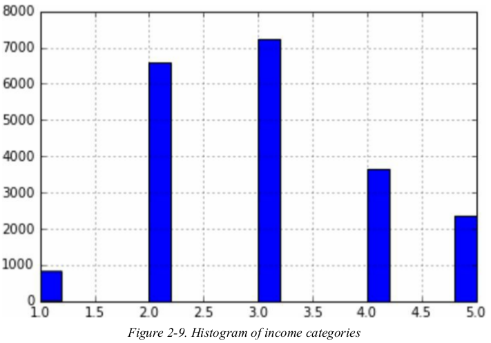
　　most median income values are clustered around 2-5(tens of thousands of dollars)，but some median incomes go far beyond 6. it is important to have a sufficient number of instances in your dataset for each stratum，or else the estimate of the the stratum's importance may be biased. this means that you should not have too many strata，and each stratum should be large enough. 

　　the following codes create an income category attribute by dividing the median income by 1.5(to limit the number of income categories)，and rounding up using ceil(to have discrete categories)，and then merging all the categories greater than 5 into category 5.

housing["income_cat"] = np.ceil(housing["median_income"] / 1.5)
housing["income_cat"].where(cond=housing["income_cat"] < 5, other=5.0, inplace=True)
print(housing["income_cat"].value_counts())

　　do stratified sampling based on the income category. Scikit-Learn 提供了StratifiedShuffleSplit class.

from sklearn.model_selection import StratifiedShuffleSplit

split = StratifiedShuffleSplit(n_splits=1, test_size=0.2, random_state=42)
for train_index, test_index in split.split(housing, housing["income_cat"]):
    strat_train_set = housing.loc[train_index]
    strat_test_set = housing.loc[test_index]

　　compare the income category proportions in the overall dataset，in the test set generated with purely random sampling，and in the test set generated with stratified sampling.

print(housing["income_cat"].value_counts() / len(housing))
print(test_set["income_cat"].value_counts() / len(test_set))
print(strat_test_set["income_cat"].value_counts() / len(strat_test_set))

#        overall   purely    stratified
# 1.0    0.039826  0.040213  0.039729
# 2.0    0.318847  0.324370  0.318798
# 3.0    0.350581  0.358527  0.350533
# 4.0    0.176308  0.167393  0.176357
# 5.0    0.114438  0.109496  0.114583

　　从结果看，the test set generated using stratified sampling has income category proportions almost identical to those in the full dataset，whereas the test set generated using purely random sampling is quite skewed.

　　(分割好测试集之后)删掉income_cat attribute，让数据回到原始状态。

for set in (strat_train_set, strat_test_set):
    set.drop(['income_cat'], axis=1, inplace=True)

Discover and Visualize the Data to Gain Insights

　　Visualizing Geographical Data

　　Looking for Correlations

　　Experimenting with Attribute Combination

　　 first，make sure you have put the test set aside and you are only exploring the training set. if the training set is very large，you may want to sample an exploring set，to make manipulation easy and fast.

　　creat a copy so you can play with it without harming the training set.

housing = strat_train_set.copy()

visualizing geographical data: 

　　since there is geographical information(latitude and longitude)，it is a good idea to create a scatterplot of all districts to visualize the data. setting the alpha option to 0.1 makes it much easier to visualize the places where there is a high density of data points.

housing.plot(kind='scatter', x='longitude', y='latitude')
housing.plot(kind='scatter', x='longitude', y='latitude', alpha=0.1)
plt.show()

　　只有这些还不够，you may need to play around with visualization parameters to make the patterns stand out.

　　加了个population attribute：look at the housing prices. the radius of each circle represents the district's population(option s)，and the color represents the price(option c).

housing.plot(kind='scatter', x='longitude', y='latitude', alpha=0.4,
             s=housing['population']/100, label='population',
             c='median_house_value', cmap=plt.get_cmap('jet'), colorbar=True)
plt.legend()
plt.show()

　　

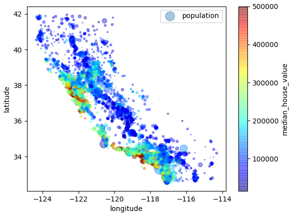
　　this image tells you that the housing prices are very much related to the location(e.g., close to the ocean) and to the population density. it will probably be useful to use a clustering algorithm to detect the main clusters，and add new features that measure the proximity to the cluster centers.

looking for correlations: 相关系数

　　since the dataset is not too large，you can easily compute the standard correlation coefficient(i.e., Pearson's r) between every pair of attributes using the corr() method: 

corr_matrix = housing.corr()

　　look at how much each attribute correlates with the median house value: 

print(corr_matrix['median_house_value'].sort_values(ascending=False))  # 数值降序显示

# median_house_value    1.000000
# median_income         0.687160
# total_rooms           0.135097
# housing_median_age    0.114110
# households            0.064506
# total_bedrooms        0.047689
# population           -0.026920
# longitude            -0.047432
# latitude             -0.142724
# Name: median_house_value, dtype: float64

　　正相关：the median house value tends to go up when the median income goes up.

　　负相关：between the latitude and the median house value(i.e., prices have a slight tendency to go down when you go north).

　　

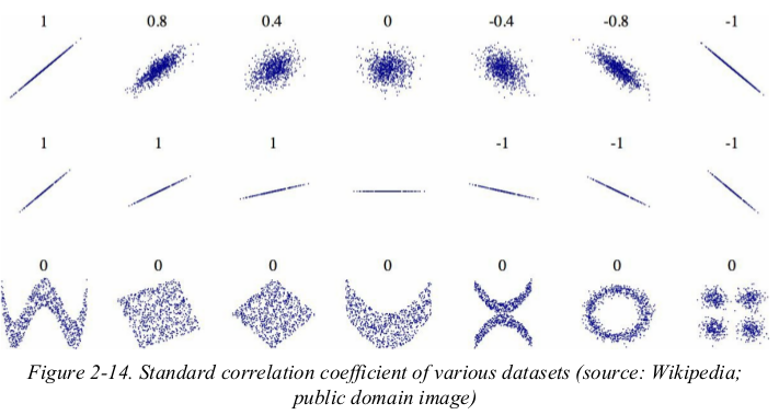
　　注意：the correlation coefficient only measures linear correlations. coefficients close to zero means that there is no linear correlation(不排除非线性相关). 如图第3行

　　注意：the second row shows examples where the correlation coefficient is equal to 1 or -1；notice that this has nothing to do with the slope. 如图第2行

　　another way to check for correlations between attributes is to use Pandas's scatter_matrix function，which plots every numerical attribute against every other numerical attribute. 下面实现只展示 a few promising attributes.

from pandas.plotting import scatter_matrix

attributes = ['median_house_value', 'median_income', 'total_rooms', 'housing_median_age']
scatter_matrix(housing[attributes], figsize=(12, 8))
plt.show()

　　

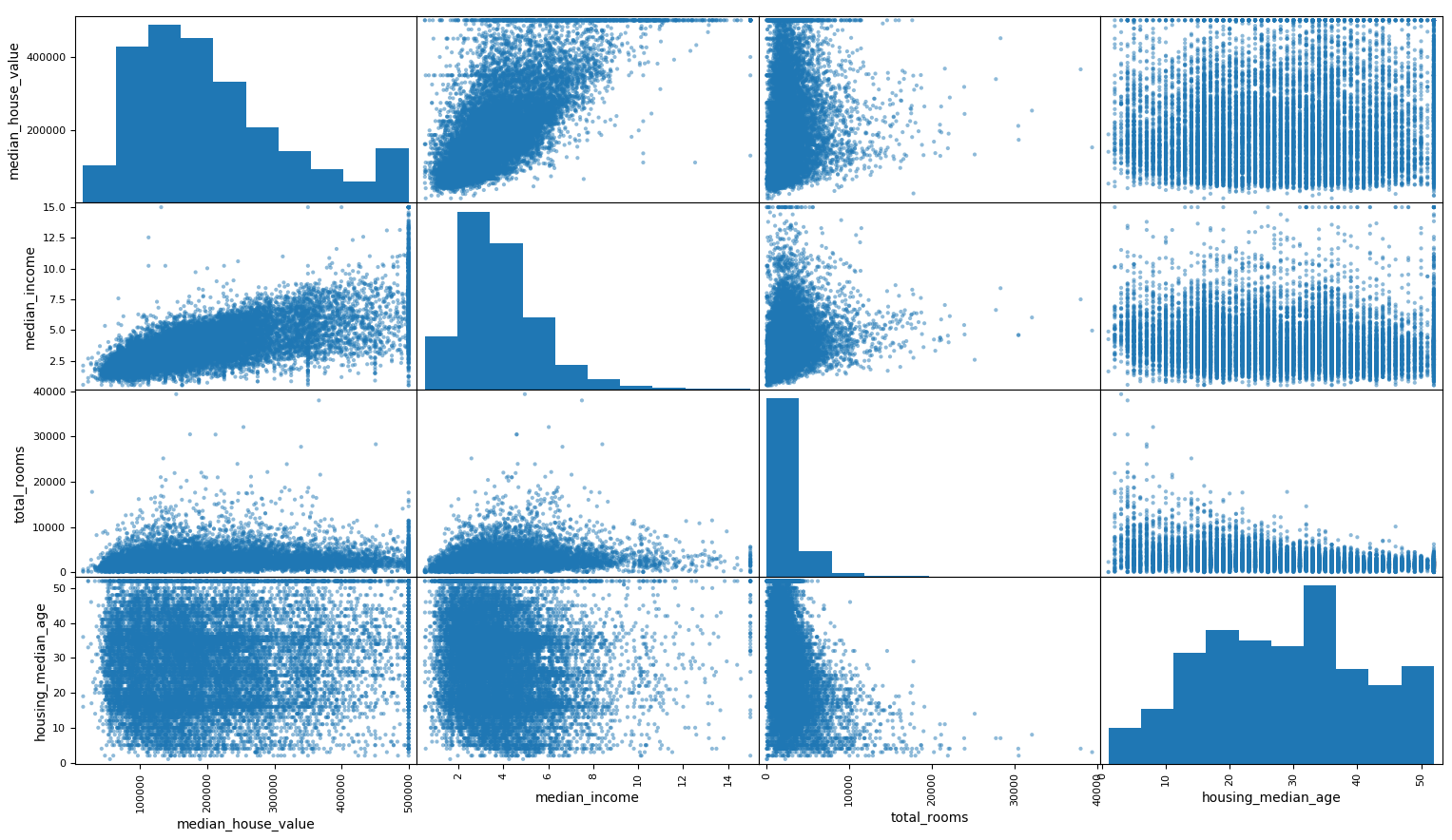
　　主对角线上以每个属性的直方图显示。

　　如图，the most promising attribute to predict the median house value is the median income，so let's zoom in on their correlation scatterplot.

housing.plot(kind='scatter', x='median_income', y='median_house_value', alpha=0.1)
plt.show()

　　

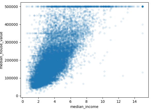
　　the price cap that we noticed earlier is clearly visible as a horizonal line at $500,000. other less obvious straight lines: $450,000，$350,000，$280,000. you may want to try removing the corresponding districts to prevent your algorithm from learning to reproduce these data quirks. 这里考虑直接删掉这些数据。

experimenting with attribute combination: 

　　for example，the total number of rooms in a district is not very useful if you don't know how many households there are. what you really want is the number of rooms per household. similarly，the total number of bedrooms by itself is not useful: you probably want to compare it to the number of rooms. and the population per household also seems like an interesting attribute combination to look at.

housing['rooms_per_household'] = housing['total_rooms'] / housing['households']
housing['bedrooms_per_room'] = housing['total_bedrooms'] / housing['total_rooms']
housing['population_per_household'] = housing['population'] / housing['households']

corr_matrix = housing.corr()
print(corr_matrix['median_house_value'].sort_values(ascending=False))

# median_house_value          1.000000
# median_income               0.687160
# rooms_per_household         0.146285
# total_rooms                 0.135097
# housing_median_age          0.114110
# households                  0.064506
# total_bedrooms              0.047689
# population_per_household   -0.021985
# population                 -0.026920
# longitude                  -0.047432
# latitude                   -0.142724
# bedrooms_per_room          -0.259984
# Name: median_house_value, dtype: float64

　　

Prepare the Data for Machine Learning Algorithm

　　Data Cleaning

　　Handling Text and Categorical Attributes

　　Custom Transformers

　　Feature Scaling

　　Transformation Pipelines

　　 separate the predictors and labels since we don't necessarily want to apply the same transformation to the predictors and the target values.  drop() creates a copy of the data and does not affect the original data.

housing = strat_train_set.drop('median_house_value', axis=1)
housing_labels = strat_train_set['median_house_value'].copy()

data cleaning: 

　　most machine learning algorithms can't work with missing features. e.g., total_bedroom attribute.

　　three options: 

　　　　get rid of the corresponding districts.

　　　　get rid of the whole attribute.

　　　　set the values to some value(zero，themean，the median，etc.)

　　使用Pandas提供的方法：DataFrame's dropna()，drop()，fillna() methods: 

housing = housing.dropna(subset=['total_bedrooms'])                   # 删掉相应数据

housing = housing.drop('total_bedrooms', axis=1)                      # 删掉相应属性

median = housing['total_bedrooms'].median()
housing['total_bedrooms'] = housing['total_bedrooms'].fillna(median)  # 填充缺失值

　　Scikit-Learn 提供的方法：SimpleImputer.

　　　　first，create an Imputer instance，specifying that you want to replace each attribute's missing values with the median of that attribute.

　　　　second，since the median can only be computed on numerical attributes，we need to create a copy of the data without the text attribute ocean_proximity. 

　　　　third，fit the imputer instance to the training data using the fit() method.

from sklearn.impute import SimpleImputer
imputer = SimpleImputer(strategy='median')
housing_num = housing.drop('ocean_proximity', axis=1)
imputer.fit(housing_num)

　　　　the imputer has simply computed the median of each attribute and stored the result in its statistics_ instance variable. 

　　　　only the total_bedrooms attribute had missing value，but we can't be sure that there won't be any missing values in new data after the system goes live，so it is safer to apply the imputer to all the numerical attributes.  上面的方法已经应用到所有数值属性了。

print(imputer.statistics_)
print(housing_num.median().values)

# [-118.51     34.26     29.     2119.5     433.     1164.      408.     3.5409]
# [-118.51     34.26     29.     2119.5     433.     1164.      408.     3.5409]

　　　　forth，you can use this "trained" imputer to transform the training set by replacing missing values by the learned medians.  the result is a plain Numpy array containing the transformed features，you can put it back into a Pandas DataFrame.

from sklearn.impute import SimpleImputer
imputer = SimpleImputer(strategy='median')
housing_num = housing.drop('ocean_proximity', axis=1)
imputer.fit(housing_num)
print(imputer.statistics_)
print(housing_num.median().values)

X = imputer.transform(housing_num)
housing_tr = pd.DataFrame(X, columns=housing_num.columns)

#################################################################################

Scikit-Learn design: 

the main design principles are: 

　　Consistency. all objects share a consistent and simple interface:

　　　　Estimators. any object that can estimate some parameters based on a dataset is called an estimator(e.g., an imputer is an estimator). the estimation itself is preformed by the fit() method，and it takes only a dataset as a parameter(or two for supervised learning algorithms；the second dataset contains the labels). any other parameter needed to guide the estimation process is considered a hyperparameter(such as an imputer's strategy)，and it must be set as an instance variable(generally via a constructor parameter). 最后一句？？

　　　　Transformers. some estimators(such as an imputer) can also transform a dataset；these are called transformers. the transformation is performed by the transform() method with the dataset to tranform as a parameter. it returned the transformed dataset. this transformation generally relies on the learned parameters， as is the case for an imputer. all transformers also have a convenience method called fit_transform() that is equivalent to calling fit() and then transform() (but sometimes fit_transform() is optimized and runs much faster).

　　　　Predictors. some estimators are capable of making predictions given a dataset；they are called predictors. for example，the LinearRegression model is a predictor: it predicts life satisfaction given a country's GDP per capita.  a predictor has a predict() method that takes a dataset of new instances and returns a dataset of corresponding predictions. it also has a score() method that measures the quality of predictions given a test set.

　　Inspection. all the estimator's hyperparameters are accessible directly via public instance variables(e.g., imputer.strategy)，and all the estimator's learned parameters are also accessible via public instance variables with an underscore suffix(e.g., imputer.statistics_)

　　Nonproliferation of classes. datasets are represented as NumPy arrays or SciPy spare matrices，instead of homemade classes. Hyperparameters are just regular strings or numbers.

　　Composition.  Existing building blocks are reused as much as possible. for example，it is easy to create a Pipeline estimator from an arbitrary sequence of transformers followed by a final estimator.

　　Sensible defaults.

#################################################################################

handling text and categorical attributes: 

 　　most machine learning algorithms prefer to work with numbers anyway，so let's convert these text label to numbers.

　　Scikt-Learn provides a transformer for this task called OrdinalEncoder.

from sklearn.preprocessing import OrdinalEncoder
ordinal_encoder = OrdinalEncoder()
housing_cat = housing[['ocean_proximity']]  # 注意是2D
housing_cat_encoded = ordinal_encoder.fit_transform(housing_cat)
print(housing_cat_encoded)

# [0 0 4 ... 1 0 3]

　　look at the mapping that this encoder has learned using the classes_ attribute.

print(encoder.categories_)

# [array(['<1H OCEAN' 'INLAND' 'ISLAND' 'NEAR BAY' 'NEAR OCEAN'], dtype=object)]

　　使用OrdinalEncoder有个问题：ML algorithm will assume that two nearby values are more similar than two distant values. obviously this is not the case. to fix this issue，a common solution is one-hot encoding. Scikit-Learn provides a OneHotEncoder to convert integer categorical values into one-hot vectors. 注意：其fit_transform() expects a 2D array.

from sklearn.preprocessing import OneHotEncoder
encoder = OneHotEncoder(categories='auto')
housing_cat_1hot = encoder.fit_transform(housing_cat_encoded)
print(housing_cat_1hot)

　　注意：the output is a SciPy sparse matrix，this is very useful when you have categorical attributes with thousands of categories. the sparse matrix only stores the location of the nonzero elements. you can use it mostly like a normal 2D array，but if you really want to convert it to a dense NumPy array，just call the toarray() method.

housing_cat_1hot_dense = housing_cat_1hot.toarray()

　　we can apply both transformations(from text categories to integer categories，then from integer categories to one-hot vectors) in one shot using LabelBinarizer class.  this returns a dense NumPy array by default，you can get a sparse matrix instead by set sparse_output=True.  用不到了，OneHotEncoder可以处理字符串了。

from sklearn.preprocessing import LabelBinarizer
housing_cat = housing['ocean_proximity']
# encoder = LabelBinarizer()
encoder = LabelBinarizer(sparse_output=True)
housing_cat_1hot = encoder.fit_transform(housing_cat)
print(housing_cat_1hot)

custom transformers: 

　　# 做的事情就是把前面线性相关的几个属性加上。

　　all you need is to create a class and implement three methods: fit() (returning self)，transform()，and fit_transform(). 

from sklearn.base import BaseEstimator, TransformerMixin

rooms_ix, bedrooms_ix, population_ix, household_ix = 3, 4, 5, 6  # 表示housing的第几个属性


class CombinedAttributesAdder(BaseEstimator, TransformerMixin):
    def __init__(self, add_bedrooms_per_room=True):
        self.add_bedrooms_per_room = add_bedrooms_per_room

    def fit(self, X, y=None):
        return self

    def transform(self, X, y=None):
        rooms_per_household = X[:, rooms_ix] / X[:, household_ix]
        population_per_household = X[:, population_ix] / X[:, household_ix]
        if self.add_bedrooms_per_room:
            bedrooms_per_room = X[:, bedrooms_ix] / X[:, rooms_ix]
            return np.c_[X, rooms_per_household, population_per_household, bedrooms_per_room]
        else:
            return np.c_[X, rooms_per_household, population_per_household]


attr_adder = CombinedAttributesAdder(add_bedrooms_per_room=False)
housing_extra_attribs = attr_adder.transform(housing.values)

　　下面的方法更简单，但不推荐: 

from sklearn.preprocessing import FunctionTransformer


def add_extra_features(X, add_bedrooms_per_room=True):
    rooms_per_household = X[:, rooms_ix] / X[:, household_ix]
    population_per_household = X[:, population_ix] / X[:, household_ix]
    if add_bedrooms_per_room:
        bedrooms_per_room = X[:, bedrooms_ix] / X[:, rooms_ix]
        return np.c_[X, rooms_per_household, population_per_household, bedrooms_per_room]
    else:
        return np.c_[X, rooms_per_household, population_per_household]


attr_adder = FunctionTransformer(add_extra_features, validate=False, kw_args={'add_bedrooms_per_room': False})
housing_extra_attribs = attr_adder.fit_transform(housing.values)
print(housing_extra_attribs)

feature scaling: 

　　machine learning algorithms don't perform well when the input numerical attributes have very different scales. this is the case for the housing data: the total number of rooms ranges from about 6 to 39320，while the median incomes only range from 0 to 15. 

　　Note that scaling the target values is generally not required.

　　there are two common ways to get all attributes to have the same scale: min-max scaling(i.e., normalization) and standardization.

　　min-max scaling: values are shifted and rescaled so that they end up ranging from 0 to 1. we do this by subtracting the min value and dividing by the max minus the min. Scikit-Learn provides a transformer called MinMaxScaler for this. it has a feature_range hyperparameter that lets you change the range if you don't want 0-1 for some reason.

　　standardization: first it subtracts the mean value，and then it divide by the variance so that the resulting distribution has unit variance. unlike min-max scaling，standardization does not bound values to a specific range，which may be a problem for some algorithms(e.g., neutral networks often expect an input value ranging from 0 to 1). however，standardization is much less affected by outliers. Scikit-Learn provides a transformer called StandardScaler for standardization.

transformation pipelines: 

　　a pipeline for numerical values: 

　　there are many data transformation steps that need to be executed in the right order. Scikit-Learn provides the Pipeline class to help with such sequences of transformations. 

from sklearn.pipeline import Pipeline
from sklearn.preprocessing import StandardScaler

num_pipeline = Pipeline([
    ('imputer', SimpleImputer(strategy='median')),
    ('attribs_adder', CombinedAttributesAdder()),
    ('std_scaler', StandardScaler()),
])
housing_num_tr = num_pipeline.fit_transform(housing_num)  # StandardScaler is a transformer

　　the Pipeline constructor takes a list of name/ estimator paris defining a sequence of steps. all but the last estimator must be transformers(i.e., they must have a fit_transform() method). 

　　when you call the pipeline's fit() method，it calls fit_transform() sequentially on all transformers，passing the output of each call as the parameter to the next call，until it reaches the final estimator，for which it just calls the fit() method.

　　the pipeline exposes the same methods as the final estimator. in this example，the last estimator is a StandardScaler，which is a transformer，so the pipeline has a transform() method that applies all the transforms to the data in sequence(it also has a fit_transform() method that we could have used instead of calling fit() and then transform()).

　　

　　a pipeline for categories values:

　　you now have a pipeline for numerical values，and you also need to apply the LabelBinarizer on the categorical values: how can you join these transformation into a single pipeline？Scikit-Learn provides a ColumnTransformer class.

　　you give it a list of transformers，and when its transform() method is called it runs each transformer's transform() method in parallel，waits for their output，and then concatenates them and returns the result. a full pipeline handling both numerical and categories attributes may look like this: 

from sklearn.pipeline import Pipeline
from sklearn.preprocessing import StandardScaler
from sklearn.compose import ColumnTransformer

num_attribs = list(housing_num)
cat_attribs = ['ocean_proximity']

num_pipeline = Pipeline([
    ('imputer', SimpleImputer(strategy='median')),
    ('attribs_adder', CombinedAttributesAdder()),
    ('std_scaler', StandardScaler()),
])

full_pipeline = ColumnTransformer(transformers=[
    ('num_pipeline', num_pipeline, num_attribs),
    ('cat_pipeline', OneHotEncoder(), cat_attribs),  # OneHotEncoder可以处理字符串了
])

housing_prepared = full_pipeline.fit_transform(housing)
print(housing_prepared)

Select and Train a Model: 

　　Training and Evaluating on the Training Set

　　Better Evaluation Using Cross-Validation

training and evaluating on the training set: 

　　使用LinearRegression 训练. (underfit)

from sklearn.linear_model import LinearRegression
from sklearn.metrics import mean_squared_error

lin_reg = LinearRegression()
lin_reg.fit(housing_prepared, housing_labels)

some_data = housing.iloc[:5]
some_labels = housing_labels.iloc[:5]
some_data_prepared = full_pipeline.transform(some_data)
print('Predictions:	', lin_reg.predict(some_data_prepared))
print('Labels:	', list(some_labels))

housing_predictions = lin_reg.predict(housing_prepared)
lin_mse = mean_squared_error(housing_labels, housing_predictions)
lin_rmse = np.sqrt(lin_mse)
print(lin_rmse)  # 68628.19819848922

　　most districts' median_housing_values range between $120,000 and $265,000，so a typical prediction error of $68,628 is not very satisfying. this is an example of a model underfitting the training set. 根据处理欠拟合的方法：you could try to add more features(e.g., the log of the population)，try a more complex model.

　　使用DecisionTreeRegressor 训练. (overfit)

　　capable of finding complex nonlinear relationships in the data.

from sklearn.tree import DecisionTreeRegressor

tree_reg = DecisionTreeRegressor()
tree_reg.fit(housing_prepared, housing_labels)

housing_predictions = tree_reg.predict(housing_prepared)
tree_mse = mean_squared_error(housing_labels, housing_predictions)
tree_rmse = np.sqrt(tree_mse)
print(tree_rmse)  # 0.0

　　could this model really be absolutely perfect or overfit？确定方法：使用分割出来的validation set.

better evaluation using cross-validation: 

　　one way to evaluate the Decision Tree model would be to use the train_test_split function to split the training set into a smaller training set and a validation set，then train your model against the smaller training set and evaluate them against the validation set.  the following code performs K-fold cross-validation: it randomly split the training set into 10 distinct subsets called folds，then it trains and evaluates the Decision Tree model 10 times，picking a different fold for evaluation every time and training on the other 9 folds. 

from sklearn.model_selection import cross_val_score
from sklearn.tree import DecisionTreeRegressor


def display_scores(scores):
    print('Scores:', scores)
    print('Mean:', scores.mean())
    print('Standard deviation:', scores.std())


tree_reg = DecisionTreeRegressor()
scores = cross_val_score(tree_reg, housing_prepared, housing_labels,
                         scoring='neg_mean_squared_error', cv=10)
tree_rmse_scores = np.sqrt(-scores)
display_scores(tree_rmse_scores)

# Scores: [69517.59475954 67330.93677783 72770.97315978 69511.33190373
#  71298.87089793 74993.78781487 71473.87594172 72632.42379012
#  76120.91423871 69970.12194439]
# Mean: 71562.0831228634
# Standard deviation: 2531.1281417742257

　　上述，Scikit-Learn cross-validation features expect a utility function(greater is better) rather than a cost function(lower is better)，so the scoring function is actually the opposite of the MSE.

　　实际上还不如LinearRegression 呢。

　　cross-validation allows you to get not only an estimate of the performance of your model，but also a measure of how precise this estimate is(i.e., its standard deviation). but cross-validation comes at the cost of training the model several times，so it is not always possible. 

　　下面是Linear Regression model

from sklearn.linear_model import LinearRegression

lin_reg = LinearRegression()
lin_scores = cross_val_score(lin_reg, housing_prepared, housing_labels,
                             scoring='neg_mean_squared_error', cv=10)
lin_rmse_scores = np.sqrt(-lin_scores)
display_scores(lin_rmse_scores)

# Scores: [66782.73843989 66960.118071   70347.95244419 74739.57052552
#  68031.13388938 71193.84183426 64969.63056405 68281.61137997
#  71552.91566558 67665.10082067]
# Mean: 69052.46136345083
# Standard deviation: 2731.674001798348

　　对比LinearRegression 和 DecisionTree 的交叉验证结果，the Decision Tree model is overfitting so badly that it performs worse than the Linear Regression model.

　　下面看一下RandomForestRegressor 怎么样. Random Forests work by training many Decision Trees on random subsets of the features，then averaging out their predictions. building a model on top of many other models is called Ensemble Learning. 

from sklearn.ensemble import RandomForestRegressor
from sklearn.metrics import mean_squared_error

forest_reg = RandomForestRegressor(n_estimators=10)
forest_reg.fit(housing_prepared, housing_labels)
housing_predictions = forest_reg.predict(housing_prepared)
forest_mse = mean_squared_error(housing_labels, housing_predictions)
forest_rmse = np.sqrt(forest_mse)
print(forest_rmse)  # 22151.378302014353


forest_scores = cross_val_score(forest_reg, housing_prepared, housing_labels,
                                scoring='neg_mean_squared_error', cv=10)
forest_rmse_scores = np.sqrt(-forest_scores)
display_scores(forest_rmse_scores)

# Scores: [51681.09152466 50542.72567963 53162.91534117 53812.84309686
#  52433.51935862 56623.59838631 51752.53148758 50948.00442038
#  56419.75801431 52365.21941861]
# Mean: 52974.22067281119
# Standard deviation: 1994.3481796509845

　　Random Forests look very promising. however，note that the score on the training set is still much lower than on the validation set，meaning that the model is still overfitting the training set.

　　before you dive much deeper in Random Forests，you should try out many other models from various categories of ML algorithms.

　　

　　you should save every model you experiment with，so you can come back easily to any model you want. make sure you save both the hyperparameters and the trained parameters，as well as the cross-validation scores and perhaps the actual predictions as well. this will allow you to easily compare scores across model types，and compare the types of errors they make.

from sklearn.externals import joblib

joblib.dump(tree_reg, 'tree_reg_model.pkl')

tree_reg_loaded = joblib.load('tree_reg_model.pkl')

Fine-Tune Your Model

　　Grid Search

　　Randomized Search

　　Ensemble Methods

　　Analyze the Best Models and Their Errors

　　Evaluate Your System on the Test Set

grid search: 

　　Scikit-Learn's GridSearchCV. tell it which hyperparameters you want it to experiment with，and what values to try out，and it will evaluate all the possible combinations for hyperparameter values，using cross-validation. 

from sklearn.ensemble import RandomForestRegressor
from sklearn.model_selection import GridSearchCV

param_grid = [
    {'n_estimators': [3, 10, 30], 'max_features': [2, 4, 6, 8]},
    {'bootstrap': [False], 'n_estimators': [3, 10], 'max_features': [2, 3, 4]}
]
forest_reg = RandomForestRegressor()
grid_search = GridSearchCV(forest_reg, param_grid, scoring='neg_mean_squared_error', cv=5)
grid_search.fit(housing_prepared, housing_labels)

　　when you have no idea what value a hyperparameter should have，a simple approach is to try out consecutive powers of 10(or a smaller number if you want a more fine-grained search，as shown in this example with the n_estimators hyperparameter). 

　　this param_grid tells Scikit-Learn to first evaluate all 3 × 4 = 12 combinations of n_estimators and max_features hyperparameter valuesspecified in the first dict，then try all 2 × 3 = 6 combinations of hyperparameter values in the second dict，but this time with the bootstrap hyperparameter set to False.

　　all in all，the grid search will explore 12 + 6 = 18 combinations of RandomForestRegressor hyperparameter values，and it will train each model five times(since cv=5). in other words，there will be 18 × 5 = 90 rounds of training. 很费时间

　　you can get the best combination of parameters like this: 

print(grid_search.best_params_)

# {'max_features': 6, 'n_estimators': 30}

　　since 30 is the maximum value of n_estimators that was evaluated，you should probably evaluate higher values as well，since the score may continue to improve.

　　you can also get the best estimator directly: 

print(grid_search.best_estimator_)

# RandomForestRegressor(bootstrap=False, criterion='mse', max_depth=None,
#            max_features=6, max_leaf_nodes=None, min_impurity_decrease=0.0,
#            min_impurity_split=None, min_samples_leaf=1,
#            min_samples_split=2, min_weight_fraction_leaf=0.0,
#            n_estimators=30, n_jobs=None, oob_score=False,
#            random_state=None, verbose=0, warm_start=False)

　　if GridSearchCV is initialized with refit=True(which is the default)，then once it finds the best estimator using cross-validation，it retrains it on the whole training set. this is usually a good idea since feeding it more data will likely improve its preformance. 

　　the evaluation score are also available: 

cvers = grid_search.cv_results_
for mean_score, params in zip(cvers['mean_test_score'], cvers['params']):
    print(np.sqrt(-mean_score), params)

# 64328.076653238946 {'n_estimators': 3, 'max_features': 2}
# 55812.895986379335 {'n_estimators': 10, 'max_features': 2}
# 53192.525517898466 {'n_estimators': 30, 'max_features': 2}
# 60945.14547566097 {'n_estimators': 3, 'max_features': 4}
# 53352.561107299065 {'n_estimators': 10, 'max_features': 4}
# 50567.59791304603 {'n_estimators': 30, 'max_features': 4}
# 59103.048274410496 {'n_estimators': 3, 'max_features': 6}
# 52072.183723235976 {'n_estimators': 10, 'max_features': 6}
# 49977.40503422386 {'n_estimators': 30, 'max_features': 6}  # best
# 58763.82955458445 {'n_estimators': 3, 'max_features': 8}
# 52298.40043582782 {'n_estimators': 10, 'max_features': 8}
# 49990.82850677243 {'n_estimators': 30, 'max_features': 8}
# 62675.0158288148 {'n_estimators': 3, 'bootstrap': False, 'max_features': 2}
# 54026.17058642057 {'n_estimators': 10, 'bootstrap': False, 'max_features': 2}
# 58625.18025776166 {'n_estimators': 3, 'bootstrap': False, 'max_features': 3}
# 52378.80079941108 {'n_estimators': 10, 'bootstrap': False, 'max_features': 3}
# 58771.92785854996 {'n_estimators': 3, 'bootstrap': False, 'max_features': 4}
# 51461.23847889301 {'n_estimators': 10, 'bootstrap': False, 'max_features': 4}

 　　the RMSE for this combination is 49977，which is slightly better than the 52974(default hyperparameter values). 

random search: 

　　the grid search approach is fine when you are exploring relatively few combinations，like in the previous example，but when the hyperparameter search space is large，it is often preferable to use RandomizedSearchCV. this class can be used in much the same way as the GridSearchCV，but instead of trying out all possible combinations，it evaluates a given number of random combinations by selecting a random value for each hyperparameter at every iteration. 

　　见习题2

ensemble methods: 

　　another way to fine-tune your system is to try to combine the combine the models that performs best. the group(or ensemble) will often perform better than the best individual model(just like Random Forests perform better than the individual Decision Trees they rely on)，especially if the individual models make very different types of errors.  

analyze the best models and their errors: 

　　you will often gain good insights on the problem by inspecting the best models. for example，the RandomForestRegressor can indicate the relative importance of each attribute for making accurate predictions: 

feature_importances = grid_search.best_estimator_.feature_importances_
print(feature_importances)

# [7.33442355e-02 6.29090705e-02 4.11437985e-02 1.46726854e-02
#  1.41064835e-02 1.48742809e-02 1.42575993e-02 3.66158981e-01
#  5.64191792e-02 1.08792957e-01 5.33510773e-02 1.03114883e-02
#  1.64780994e-01 6.02803867e-05 1.96041560e-03 2.85647464e-03]

extra_attribs = ["rooms_per_household", "population_per_household", "bedrooms_per_room"]  # 这个顺序很重要，与创建时一一对应
cat_encoder = full_pipeline.named_transformers_['cat_pipeline']
cat_one_hot_attribs = list(cat_encoder.categories_[0])
attributes = num_attribs + extra_attribs + cat_one_hot_attribs
print(sorted(zip(feature_importances, attributes), reverse=True))

# [(0.3661589806181342, 'median_income'), 
#  (0.1647809935615905, 'INLAND'), 
#  (0.10879295677551573, 'population_per_household'), 
#  (0.07334423551601242, 'longitude'), 
#  (0.0629090704826203, 'latitude'), 
#  (0.05641917918195401, 'rooms_per_household'), 
#  (0.05335107734767581, 'bedrooms_per_room'), 
#  (0.041143798478729635, 'housing_median_age'), 
#  (0.014874280890402767, 'population'), 
#  (0.014672685420543237, 'total_rooms'), 
#  (0.014257599323407807, 'households'), 
#  (0.014106483453584102, 'total_bedrooms'), 
#  (0.010311488326303787, '<1H OCEAN'), 
#  (0.002856474637320158, 'NEAR OCEAN'), 
#  (0.00196041559947807, 'NEAR BAY'), 
#  (6.028038672736599e-05, 'ISLAND')]

　　with this information，you may want to try dropping some of the less useful features(e.g., apparently only one ocean_proximity category is really useful，so you could try dropping the others). 

　　you should also look at the specific errors that your systems makes，then try to understand why it makes them and what could fix the problem. 

evaluate your system on the test set: 

from sklearn.metrics import mean_squared_error

X_test = strat_test_set.drop('median_house_value', axis=1)
y_test = strat_test_set['median_house_value'].copy()

X_test_prepared = full_pipeline.transform(X_test)
final_model = grid_search.best_estimator_
final_predictions = final_model.predict(X_test_prepared)
final_mse = mean_squared_error(y_test, final_predictions)
final_rmse = np.sqrt(final_mse)
print(final_rmse)  # 47730.22690385927

　　the performance will usually be slightly worse than what you measured using cross-validation if you did a lot of hyperparameter tuning. but it is not the case in this example. 　　

Launch，Monitor，and Maintain Your System

　　you need to write monitoring code to check your system's live performance at regular intervals and trigger alerts when it drops. this is important to catch not only sudden breakage，but also performance degradation. 　　Evaluating your system's performance will require sampling the system's predictions and evaluating them. this will generally require a human analysis. 

 　　you should also make sure you evaluate the system's input data quality. sometimes performance will degrade slightly because of a poor quality signal，but it may take a while before your system's performance degrades enough to trigger an alert. if you monitor your system's inputs，you may catch this earlier. monitoring the inputs is particularly important for online learning systems. 

　　if your system is an online learning system，you should make sure you save snapshots of its state at regular intervals so you can easily roll back to a previously working state.

Try It Out

much of the work is in the data preparation step, building monitoring tools, setting up human evaluation pipelines, and automating regular model training. The Machine Learning algorithms are also important, of course, but it is probably preferable to be comfortable with the overall process and know three or four algorithms well rather than to spend all your time exploring advanced algorithms and not enough time on the
overall process.

1. Try a Support Vector Machine regressor (sklearn.svm.SVR)，with various hyperparameters such as kernel="linear" (with various values for the C hyperparameter) or kernel="rbf" (with various values for the C and gamma hyperparameters). How does the best SVR predictor perform?

from sklearn.svm import SVR
from sklearn.model_selection import GridSearchCV

svr_reg = SVR(kernel='linear')
svr_reg.fit(housing_prepared, housing_labels)
housing_predictions = svr_reg.predict(housing_prepared)
svr_mse = mean_squared_error(housing_labels, housing_predictions)
svr_rmse = np.sqrt(svr_mse)
print(svr_rmse)  # 111094.6308539982

svr_reg = SVR(gamma='auto')
svr_reg.fit(housing_prepared, housing_labels)
housing_predictions = svr_reg.predict(housing_prepared)
svr_mse = mean_squared_error(housing_labels, housing_predictions)
svr_rmse = np.sqrt(svr_mse)
print(svr_rmse)  # 118577.43356412371

param_grid = [
    {'kernel': ['linear'], 'C': [10., 30., 100., 300., 1000., 3000., 10000., 30000.0]},
    {'kernel': ['rbf'], 'C': [1.0, 3.0, 10., 30., 100., 300., 1000.0], 'gamma': [0.01, 0.03, 0.1, 0.3, 1.0, 3.0]},
]
svr_reg = SVR()
grid_search = GridSearchCV(svr_reg, param_grid, scoring='neg_mean_squared_error', cv=5, verbose=2, n_jobs=4)
grid_search.fit(housing_prepared, housing_labels)
neg_mse = grid_search.best_score_
grid_rmse = np.sqrt(-neg_mse)
print(grid_rmse)  # 70363.90313964167
print(grid_search.best_params_)  # {'C': 30000.0, 'kernel': 'linear'}

2. Try replacing GridSearchCV with RandomizedSearchCV .

from sklearn.svm import SVR
from sklearn.model_selection import RandomizedSearchCV
from scipy.stats import expon, reciprocal

param_distribs = {
    'kernel': ['linear', 'rbf'],
    'C': reciprocal(20, 200000),
    'gamma': expon(scale=1.0),
}

svr_reg = SVR()
rnd_search = RandomizedSearchCV(svr_reg,param_distributions=param_distribs,
                                n_iter=50, cv=5, scoring='neg_mean_squared_error',
                                verbose=2, n_jobs=4, random_state=42)
rnd_search.fit(housing_prepared, housing_labels)
neg_mse = rnd_search.best_score_
rnd_rmse = np.sqrt(-neg_mse)
print(rnd_rmse)  # 54767.99053704409
print(rnd_search.best_params_)  # {'gamma': 0.26497040005002437, 'C': 157055.10989448498, 'kernel': 'rbf'}

　　randomized search tends to find better hyperparameters than grid search in the same amount of time.

3. Try adding a transformer in the preparation pipeline to select only the most important attributes.

def indices_of_top_k(arr, k):
    return np.sort(np.argpartition(np.array(arr), -k)[-k:])


class TopFeatureSelector(BaseEstimator, TransformerMixin):
    def __init__(self, feature_importances, k):
        self.feature_importances = feature_importances
        self.k = k

    def fit(self, X, y=None):
        self.feature_indices_ = indices_of_top_k(self.feature_importances, self.k)
        return self

    def transform(self, X):
        return X[:, self.feature_indices_]


k = 5
top_k_feature_indices = indices_of_top_k(feature_importances, k)
print(top_k_feature_indices)  # [ 0  1  7  9 12]
print(housing_prepared[:3, top_k_feature_indices])

print(np.array(attributes)[top_k_feature_indices])
print(sorted(zip(feature_importances, attributes), reverse=True)[:k])


preparation_and_feature_selection_pipeline = Pipeline([
    ('preparation', full_pipeline),
    ('feature_selection', TopFeatureSelector(feature_importances, k))
])
housing_prepared_top_k_features = preparation_and_feature_selection_pipeline.fit_transform(housing)
print(housing_prepared_top_k_features[:3])

4. Try creating a single pipeline that does the full data preparation plus the final prediction.

5. Automatically explore some preparation options using GridSearchCV .

 

import matplotlib.pyplot as plt
import numpy as np
import hashlib
from sklearn.model_selection import train_test_split, StratifiedShuffleSplit
from pandas.plotting import scatter_matrix
from sklearn.impute import SimpleImputer
from sklearn.preprocessing import LabelEncoder, OneHotEncoder, LabelBinarizer, StandardScaler
from categoricalEncoder import CategoricalEncoder
from sklearn.base import BaseEstimator, TransformerMixin
from sklearn.pipeline import Pipeline, FeatureUnion
from sklearn_features.transformers import DataFrameSelector  # 第三方库 pip install sklearn-features
from sklearn.linear_model import LinearRegression
from sklearn.metrics import mean_squared_error
from sklearn.tree import DecisionTreeRegressor
from sklearn.model_selection import cross_val_score, GridSearchCV, RandomizedSearchCV
from sklearn.ensemble import RandomForestRegressor
from sklearn.svm import SVR
from scipy.stats import randint, expon, reciprocal  # expon、reciprocal还没搞定
from sklearn.base import BaseEstimator, TransformerMixin