下面内容抄袭这里的:galaxy.agh.edu.pl/~vlsi/AI/backp_t_en/backprop.html
Principles of training multi-layer neural network using backpropagation
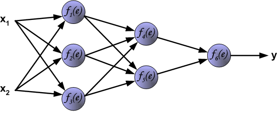
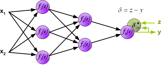
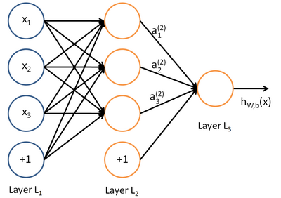
The project describes teaching process of multi-layer neural network employing backpropagation algorithm. To illustrate this process the three layer neural network with two inputs and one output,which is shown in the picture below, is used:
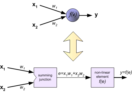
Each neuron is composed of two units. First unit adds products of weights coefficients and input signals. The second unit realise nonlinear
function, called neuron activation function. Signal e is adder output signal, and y = f(e) is output signal of nonlinear
element. Signal y is also output signal of neuron.
To teach the neural network we need training data set. The training data set consists of input signals (x1 and
x2 ) assigned with corresponding target (desired output) z. The network training is an iterative process. In each
iteration weights coefficients of nodes are modified using new data from training data set. Modification is calculated using algorithm
described below:
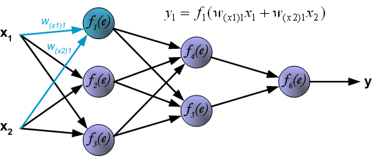
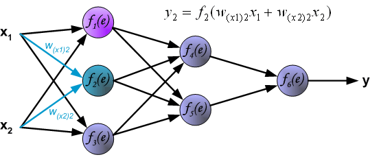
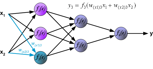
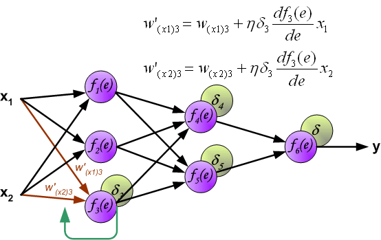
Each teaching step starts with forcing both input signals from training set. After this stage we can determine output signals values for
each neuron in each network layer. Pictures below illustrate how signal is propagating through the network, Symbols w(xm)n
represent weights of connections between network input xm and neuron n in input layer. Symbols yn
represents output signal of neuron n.
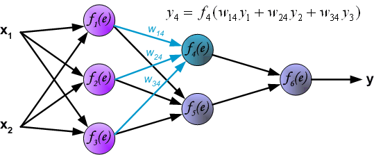
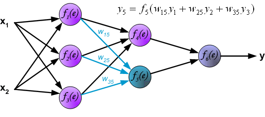
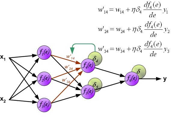
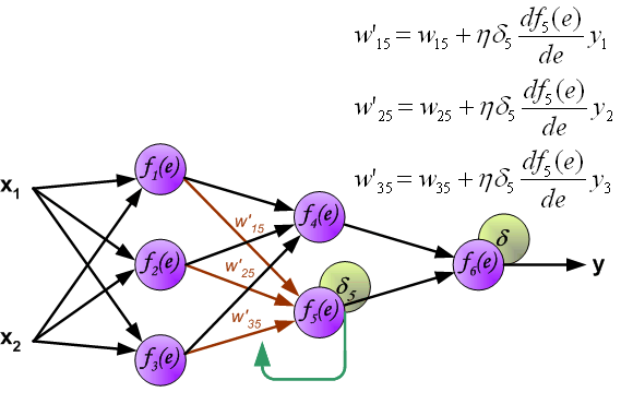
Propagation of signals through the hidden layer. Symbols wmn represent weights of connections between output of neuron
m and input of neuron n in the next layer.
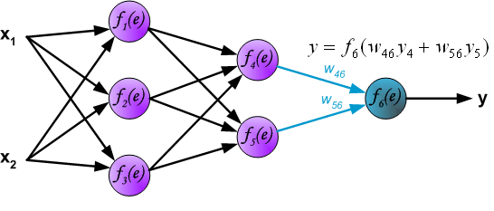
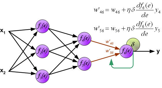
Propagation of signals through the output layer.
In the next algorithm step the output signal of the network y is compared with the desired output value (the target), which is found
in training data set. The difference is called error signal d of
output layer neuron.
下面才是反向传播部分
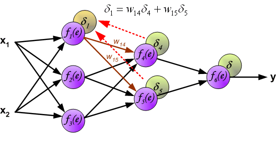
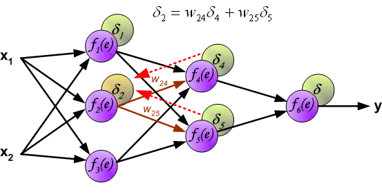
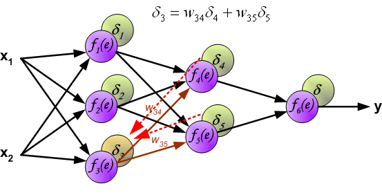
It is impossible to compute error signal for internal neurons directly, because output values of these neurons are unknown. For many years
the effective method for training multiplayer networks has been unknown. Only in the middle eighties the backpropagation algorithm has been
worked out. The idea is to propagate error signal d (computed in
single teaching step) back to all neurons, which output signals were input for discussed neuron.
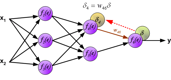
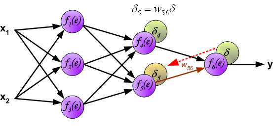
The weights' coefficients wmn used to propagate errors back are equal to this used during computing output value. Only the
direction of data flow is changed (signals are propagated from output to inputs one after the other[一个接一个地]). This technique is used for all network
layers. If propagated errors came from few[几个] neurons they are added. The illustration is below:
When the error signal for each neuron is computed, the weights coefficients of each neuron input node may be modified. In formulas below
df(e)/de represents derivative of neuron activation function (which weights are modified).
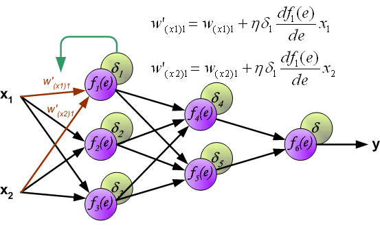
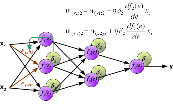
Coefficient h affects network teaching speed. There are a few
techniques to select this parameter. The first method is to start teaching process with large value of the parameter. While weights
coefficients are being established the parameter is being decreased gradually. The second, more complicated, method starts teaching with
small parameter value. During the teaching process the parameter is being increased when the teaching is advanced and then decreased again in
the final stage. Starting teaching process with low parameter value enables to determine weights coefficients signs.
通过上面的内容,最起码知道了反向传播更新参数的流程,但是没发现链式法则体现在哪里??
更新参数是从前往后进行的,那么y1、y2等是更新参数之前的取值还是更新参数之后的取值呢??私以为是前者。
下面是抄袭这里的:https://www.zhihu.com/question/27239198/answer/89853077
深度学习同样也是为了这个目的,只不过此时,样本点不再限定为(x, y)点对,而可以是由向量、矩阵等等组成的广义点对(X,Y)。而此时,(X,Y)之间的关系也变得十分复杂,不太可能用一个简单函数表示。然而,人们发现可以用多层神经网络来表示这样的关系,而多层神经网络的本质就是一个多层复合的函数。借用网上找到的一幅图[1],来直观描绘一下这种复合关系。
其对应的表达式如下:
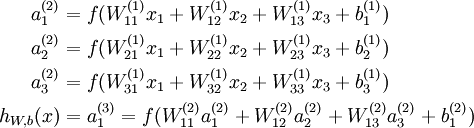 上面式中的Wij就是相邻两层神经元之间的权值,它们就是深度学习需要学习的参数,也就相当于直线拟合y=k*x+b中的待求参数k和b。
和直线拟合一样,深度学习的训练也有一个目标函数,这个目标函数定义了什么样的参数才算一组“好参数”,不过在机器学习中,一般是采用成本函数(cost function),然后,训练目标就是通过调整每一个权值Wij来使得cost达到最小。cost函数也可以看成是由所有待求权值Wij为自变量的复合函数,而且基本上是非凸的,即含有许多局部最小值。但实际中发现,采用我们常用的梯度下降法就可以有效的求解最小化cost函数的问题。
梯度下降法需要给定一个初始点,并求出该点的梯度向量,然后以负梯度方向为搜索方向,以一定的步长进行搜索,从而确定下一个迭代点,再计算该新的梯度方向,如此重复直到cost收敛。那么如何计算梯度呢?
假设我们把cost函数表示为
我们以求e=(a+b)*(b+1)的偏导为例。
它的复合关系画出图可以表示如下:
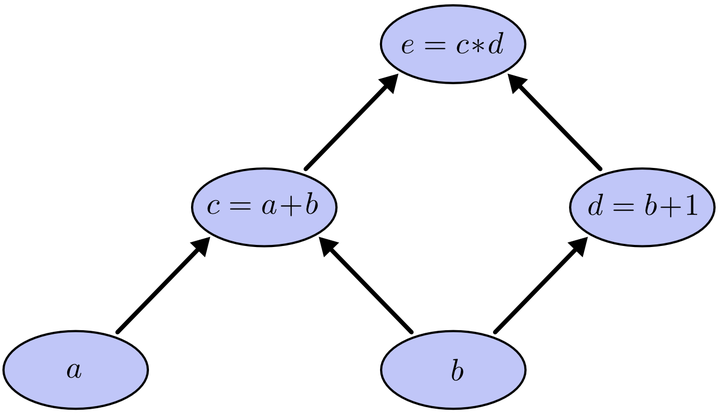 在图中,引入了中间变量c,d。
为了求出a=2, b=1时,e的梯度,我们可以先利用偏导数的定义求出不同层之间相邻节点的偏导关系,如下图所示。
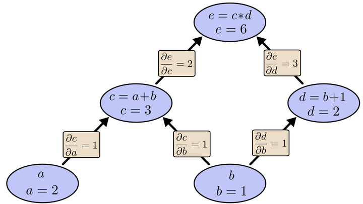 利用链式法则我们知道:
链式法则在上图中的意义是什么呢?其实不难发现,
大家也许已经注意到,这样做是十分冗余的,因为很多路径被重复访问了。比如上图中,a-c-e和b-c-e就都走了路径c-e。对于权值动则数万的深度模型中的神经网络,这样的冗余所导致的计算量是相当大的。
同样是利用链式法则,BP算法则机智地避开了这种冗余,它对于每一个路径只访问一次就能求顶点对所有下层节点的偏导值。
正如反向传播(BP)算法的名字说的那样,BP算法是反向(自上往下)来寻找路径的。
从最上层的节点e开始,初始值为1,以层为单位进行处理。对于e的下一层的所有子节点,将1乘以e到某个节点路径上的偏导值,并将结果“堆放”在该子节点中。等e所在的层按照这样传播完毕后,第二层的每一个节点都“堆放"些值,然后我们针对每个节点,把它里面所有“堆放”的值求和,就得到了顶点e对该节点的偏导。然后将这些第二层的节点各自作为起始顶点,初始值设为顶点e对它们的偏导值,以"层"为单位重复上述传播过程,即可求出顶点e对每一层节点的偏导数。
以上图为例,节点c接受e发送的1*2并堆放起来,节点d接受e发送的1*3并堆放起来,至此第二层完毕,求出各节点总堆放量并继续向下一层发送。节点c向a发送2*1并对堆放起来,节点c向b发送2*1并堆放起来,节点d向b发送3*1并堆放起来,至此第三层完毕,节点a堆放起来的量为2,节点b堆放起来的量为2*1+3*1=5, 即顶点e对b的偏导数为5.
举个不太恰当的例子,如果把上图中的箭头表示欠钱的关系,即c→e表示e欠c的钱。以a, b为例,直接计算e对它们俩的偏导相当于a, b各自去讨薪。a向c讨薪,c说e欠我钱,你向他要。于是a又跨过c去找e。b先向c讨薪,同样又转向e,b又向d讨薪,再次转向e。可以看到,追款之路,充满艰辛,而且还有重复,即a, b 都从c转向e。
而BP算法就是主动还款。e把所欠之钱还给c,d。c,d收到钱,乐呵地把钱转发给了a,b,皆大欢喜。