u版本的yolo3代码是真的复杂。
loss.py详细的代码注释如下:
# Loss functions

import torch
import torch.nn as nn

from utils.general import bbox_iou
from utils.torch_utils import is_parallel


def smooth_BCE(eps=0.1):  # https://github.com/ultralytics/yolov3/issues/238#issuecomment-598028441
    # return positive, negative label smoothing BCE targets
    return 1.0 - 0.5 * eps, 0.5 * eps


class BCEBlurWithLogitsLoss(nn.Module):
    # BCEwithLogitLoss() with reduced missing label effects.
    def __init__(self, alpha=0.05):
        super(BCEBlurWithLogitsLoss, self).__init__()
        self.loss_fcn = nn.BCEWithLogitsLoss(reduction='none')  # must be nn.BCEWithLogitsLoss()
        self.alpha = alpha

    def forward(self, pred, true):
        loss = self.loss_fcn(pred, true)
        pred = torch.sigmoid(pred)  # prob from logits
        dx = pred - true  # reduce only missing label effects
        # dx = (pred - true).abs()  # reduce missing label and false label effects
        alpha_factor = 1 - torch.exp((dx - 1) / (self.alpha + 1e-4))
        loss *= alpha_factor
        return loss.mean()


class FocalLoss(nn.Module):
    # Wraps focal loss around existing loss_fcn(), i.e. criteria = FocalLoss(nn.BCEWithLogitsLoss(), gamma=1.5)
    def __init__(self, loss_fcn, gamma=1.5, alpha=0.25):
        super(FocalLoss, self).__init__()
        self.loss_fcn = loss_fcn  # must be nn.BCEWithLogitsLoss()
        self.gamma = gamma
        self.alpha = alpha
        self.reduction = loss_fcn.reduction
        self.loss_fcn.reduction = 'none'  # required to apply FL to each element

    def forward(self, pred, true):
        loss = self.loss_fcn(pred, true)
        # p_t = torch.exp(-loss)
        # loss *= self.alpha * (1.000001 - p_t) ** self.gamma  # non-zero power for gradient stability

        # TF implementation https://github.com/tensorflow/addons/blob/v0.7.1/tensorflow_addons/losses/focal_loss.py
        pred_prob = torch.sigmoid(pred)  # prob from logits
        p_t = true * pred_prob + (1 - true) * (1 - pred_prob)
        alpha_factor = true * self.alpha + (1 - true) * (1 - self.alpha)
        modulating_factor = (1.0 - p_t) ** self.gamma
        loss *= alpha_factor * modulating_factor

        if self.reduction == 'mean':
            return loss.mean()
        elif self.reduction == 'sum':
            return loss.sum()
        else:  # 'none'
            return loss


class QFocalLoss(nn.Module):
    # Wraps Quality focal loss around existing loss_fcn(), i.e. criteria = FocalLoss(nn.BCEWithLogitsLoss(), gamma=1.5)
    def __init__(self, loss_fcn, gamma=1.5, alpha=0.25):
        super(QFocalLoss, self).__init__()
        self.loss_fcn = loss_fcn  # must be nn.BCEWithLogitsLoss()
        self.gamma = gamma
        self.alpha = alpha
        self.reduction = loss_fcn.reduction
        self.loss_fcn.reduction = 'none'  # required to apply FL to each element

    def forward(self, pred, true):
        loss = self.loss_fcn(pred, true)

        pred_prob = torch.sigmoid(pred)  # prob from logits
        alpha_factor = true * self.alpha + (1 - true) * (1 - self.alpha)
        modulating_factor = torch.abs(true - pred_prob) ** self.gamma
        loss *= alpha_factor * modulating_factor

        if self.reduction == 'mean':
            return loss.mean()
        elif self.reduction == 'sum':
            return loss.sum()
        else:  # 'none'
            return loss


class ComputeLoss:
    # Compute losses
    def __init__(self, model, autobalance=False):
        super(ComputeLoss, self).__init__()
        device = next(model.parameters()).device  # get model device
        h = model.hyp  # hyperparameters
        '''
        {'lr0': 0.01, 'lrf': 0.2, 'momentum': 0.937, 'weight_decay': 0.0005, 'warmup_epochs': 3.0, 'warmup_momentum': 0.8,
         'warmup_bias_lr': 0.1, 'box': 0.05, 'cls': 0.5, 'cls_pw': 1.0, 'obj': 1.0, 'obj_pw': 1.0, 'iou_t': 0.2,
         'anchor_t': 4.0, 'fl_gamma': 0.0, 'hsv_h': 0.015, 'hsv_s': 0.7, 'hsv_v': 0.4, 'degrees': 0.0, 'translate': 0.1,
          'scale': 0.5, 'shear': 0.0, 'perspective': 0.0, 'flipud': 0.0, 'fliplr': 0.5, 'mosaic': 1.0, 'mixup': 0.0, 'label_smoothing': 0.0}
        '''

        # Define criteria
        BCEcls = nn.BCEWithLogitsLoss(pos_weight=torch.tensor([h['cls_pw']], device=device))
        BCEobj = nn.BCEWithLogitsLoss(pos_weight=torch.tensor([h['obj_pw']], device=device))

        # Class label smoothing https://arxiv.org/pdf/1902.04103.pdf eqn 3
        #self.cp 1.0   self.cn 0.0
        self.cp, self.cn = smooth_BCE(eps=h.get('label_smoothing', 0.0))  # positive, negative BCE targets

        # Focal loss  g=0
        g = h['fl_gamma']  # focal loss gamma
        if g > 0:
            BCEcls, BCEobj = FocalLoss(BCEcls, g), FocalLoss(BCEobj, g)

        det = model.module.model[-1] if is_parallel(model) else model.model[-1]  # Detect() module
        self.balance = {3: [4.0, 1.0, 0.4]}.get(det.nl, [4.0, 1.0, 0.25, 0.06, .02])  # P3-P7
        self.ssi = list(det.stride).index(16) if autobalance else 0  # stride 16 index  autobalance = False   0
        self.BCEcls, self.BCEobj, self.gr, self.hyp, self.autobalance = BCEcls, BCEobj, model.gr, h, autobalance
        for k in 'na', 'nc', 'nl', 'anchors':
            setattr(self, k, getattr(det, k))
        '''
        na = 3
        nc = 80
        nl = 3
        anchors =
        tensor([[[1.25000, 1.62500],
                 [2.00000, 3.75000],
                 [4.12500, 2.87500]],

                [[1.87500, 3.81250],
                 [3.87500, 2.81250],
                 [3.68750, 7.43750]],

                [[3.62500, 2.81250],
                 [4.87500, 6.18750],
                 [11.65625, 10.18750]]], device='cuda:0')

        注意这里的anchor数值已经归一化到指定的缩放比例下了。
        在class Model代码有这么一段代码归一化:


        m = self.model[-1]  # Detect()
        if isinstance(m, Detect):
            s = 256  # 2x min stride
            m.inplace = self.inplace

            # tmp111 = self.forward(torch.zeros(1, ch, s, s))
            #value [8,16,32]
            m.stride = torch.tensor([s / x.shape[-2] for x in self.forward(torch.zeros(1, ch, s, s))])  # forward
            tmp12 = m.stride.view(-1, 1, 1) #shape [3,1,1]

            通过跑前向得到3层featuremap的缩放系数分别是8,16,32


            #m.anchors shape[3,3,2]

            tensor([[[ 10.,  13.],
         [ 16.,  30.],
         [ 33.,  23.]],

        [[ 30.,  61.],
         [ 62.,  45.],
         [ 59., 119.]],

        [[116.,  90.],
         [156., 198.],
         [373., 326.]]])


            m.anchors /= m.stride.view(-1, 1, 1)
            check_anchor_order(m)
            self.stride = m.stride
            self._initialize_biases()  # only run once
            # logger.info('Strides: %s' % m.stride.tolist())

            有3个featuremap,对应3组anchor,对应3个缩放系数,原本的anchor都是相对于原图大小的,分别对应了原图小中大目标。
            那么在不同缩放层的featuremap上面,anchor也要做对应的缩放

        '''

    def __call__(self, p, targets):  # predictions, targets, model

        '''
        :param p: list
        [4,3,80,80,85]
        [4,3,40,40,85]
        [4,3,20,20,85]

        :param targets:  [95,6]
        [bs,class,x,y,w,h]
        :return:
        '''
        device = targets.device
        lcls, lbox, lobj = torch.zeros(1, device=device), torch.zeros(1, device=device), torch.zeros(1, device=device)
        tcls, tbox, indices, anchors = self.build_targets(p, targets)  # targets

        '''
                看完这里总结一下函数build_targets:
                这段代码就是gt与anchor绑定
                在3个层次上大小的feature map,把gt也放到这3个大小的feature map上面
                gt的长宽与anchor长宽比小于4的,就认为gt与anchor匹配,这是重要的一步。
                然后gt在当前feature map上面取小数,就是整数部分代表一个单元格,目标的中心在这个单元格,那么就该单元格负责;
                这里比如有90个目标gt,那么传出去的变量行数都为90,列的话有b,c,x,y,w,h,a
                这里很巧妙的是a代表着是哪个anchor,一个单元格有3个anchor,只要长宽比小于4,那么都保留
                这样设计的话就是一行里面,代表一个gt,一行有gt所有信息,b,c,x,y,w,h,a
                anch是具体的anchor的值,比如(35,24)

                tcls, tbox, indices, anch
                tcls是list,有3个列表,每个shape是[95],[84],[90]
                tbox是list,有3个列表,每个shape是[95,4],[84,4],[90,4]
                indices是list,有3个列表,每个列表是元组,每个元组存放了4个shape是[95],[84],[90]的tensor
                anch是list,有3个列表,[95,2],[84,2],[90,2]
        '''

        # Losses
        for i, pi in enumerate(p):  # layer index, layer predictions
            #pi [4,3,80,80,85]  [4,3,40,40,85]  [4,3,20,20,85]
            #tmp_0 = pi[..., 0] #[4,3,80,80]
            #b[95]  a[95]  gi[95]  gj[95]
            b, a, gj, gi = indices[i]  # image, anchor, gridy, gridx
            #tobj  [4,3,80,80]
            tobj = torch.zeros_like(pi[..., 0], device=device)  # target obj

            n = b.shape[0]  # number of targets
            if n:
                ## ps [95,85]
                ps = pi[b, a, gj, gi]  # prediction subset corresponding to targets
                # 这里需要仔细看下,这里pi是网络输出的值,
                # 而b,a,gj,gi都是目标gt的信息
                #所以这里就是为了让网络输出的值相应位置也要和gt一样!

                # Regression
                pxy = ps[:, :2].sigmoid() * 2. - 0.5  #[95,2]
                pwh = (ps[:, 2:4].sigmoid() * 2) ** 2 * anchors[i] #[95,2]
                pbox = torch.cat((pxy, pwh), 1)  # predicted box  #[95,4]
                '''
                pxy加sigmod是为了让值变为0-1之间数值,pxy是小数,就是相对于某个单元格是小数坐标。
                单元格是相应位置,已经根据gj,gi获取到了,ps = pi[b, a, gj, gi]
                就是代表着坐标【gi,gj】,你这个位置来负责和目标gt一样!

                pwh同样需要sigmod把值归一化到0-1之间,然后乘上anchors[i],因为anchor的长宽与gt相差不大了,就是4倍左右。
                所以把网络预测值×2再平方
                [0-1] --> [0,2] -->[0,4]  ||||  (ps[:, 2:4].sigmoid() * 2) ** 2
                '''
                iou = bbox_iou(pbox.T, tbox[i], x1y1x2y2=False, CIoU=True)  # iou(prediction, target)  [95]
                lbox += (1.0 - iou).mean()  # iou loss  [1]
                '''
                这里一开始没看明白,x,y是相对于单元格里面的偏移,是小数。
                得到bbox还需要加上单元格的gi,gj坐标啊。
                而实际代码就是把偏移当做中心坐标来计算框交并比了。

                后来想想确实可以,因为只是个中心点坐标,计算交并比. 把两个框放到哪里计算都一样,只要你的相对位置没有变就可以!
                这里就是说你单元格gi,gj坐标一样,然后就是看你中心点小数部分的坐标了。

                lbox += (1.0 - iou).mean()  # iou loss  [1]
                ciou  loss 格式,加上一个mean就变成一个值了!
                '''

                #[95]
                #tmp_3 = (1.0 - self.gr) + self.gr * iou.detach().clamp(0).type(tobj.dtype)
                # Objectness
                tobj[b, a, gj, gi] = (1.0 - self.gr) + self.gr * iou.detach().clamp(0).type(tobj.dtype)  # iou ratio
                '''
                #tobj  [4,3,80,80]
                这里tobj[b, a, gj, gi]
                [b, a, gj, gi]可以确保得到和iou一样的个数95
                然后iou95个值就放到同样位置上去。
                代表这95个位置上才有目标,且用iou的值代表有目标的概率
                '''

                # Classification
                if self.nc > 1:  # cls loss (only if multiple classes)
                    #t [95,80]
                    t = torch.full_like(ps[:, 5:], self.cn, device=device)  # targets
                    '''
                    ps [95,85]
                    ps[:, 5:]  --> shape [95,80] 是每个类别的分数
                    self.cn = 0
                    t [95,80] 值都为0
                    '''
                    t[range(n), tcls[i]] = self.cp
                    '''
                    range(n)  -->shape[95]  值是0-94
                    tcls是list,有3个列表,每个shape是[95],[84],[90]
                    tcls[i] 存放的是95个目标的类别数
                    self.cp = 1
                    所以, t[range(n), tcls[i]] = self.cp这行代码的意思就是:
                    把每个目标的相应类别位置赋值为1
                    相当于one-hot格式的gt
                    '''

                    lcls += self.BCEcls(ps[:, 5:], t)  # BCE  [1]
                    '''
                    t [95,80]

                    ## ps [95,85]
                    ps[:, 5:]  -->[95,80]

                    '''

                # Append targets to text file
                # with open('targets.txt', 'a') as file:
                #     [file.write('%11.5g ' * 4 % tuple(x) + '
') for x in torch.cat((txy[i], twh[i]), 1)]

            obji = self.BCEobj(pi[..., 4], tobj)
            lobj += obji * self.balance[i]  # obj loss

            '''
            self.balance[i] [4,1,1]
             #tobj  [4,3,80,80]
             #pi [4,3,80,80,85]
            pi[..., 4]  -->[4,3,80,80]
             这里说下85含义,    x,y,w,h,is_obj,class_0,class_1,...,class_79
             所以,4就代表是否是目标这类
            '''

            if self.autobalance:
                self.balance[i] = self.balance[i] * 0.9999 + 0.0001 / obji.detach().item()

        if self.autobalance:
            self.balance = [x / self.balance[self.ssi] for x in self.balance]
        lbox *= self.hyp['box'] #0.05
        lobj *= self.hyp['obj'] #1.0
        lcls *= self.hyp['cls'] #0.5
        bs = tobj.shape[0]  # batch size

        loss = lbox + lobj + lcls
        return loss * bs, torch.cat((lbox, lobj, lcls, loss)).detach()
    #                          targets[bs,class,x,y,w,h]
    def build_targets(self, p, targets): #p list [4,3,80,80,85] [4,3,40,40,85] [4,3,20,20,85]  targets[31,6]
        # Build targets for compute_loss(), input targets(image,class,x,y,w,h)
        na, nt = self.na, targets.shape[0]  # number of anchors 3, targets  na = 3,nt = 31
        tcls, tbox, indices, anch = [], [], [], []
        gain = torch.ones(7, device=targets.device)  # normalized to gridspace gain
        ai = torch.arange(na, device=targets.device).float().view(na, 1).repeat(1, nt)  # same as .repeat_interleave(nt)  [3,31]
        tmp_1 = targets.repeat(na, 1, 1) # target[31,6]  tmp_1[3,31,6]
        tmp_2 = ai[:, :, None] #[3,31,1]
        targets = torch.cat((targets.repeat(na, 1, 1), ai[:, :, None]), 2)  # append anchor indices  [3,31,7]
        '''
        这里相当于把targets复制了3份,并且把每一份后面写了0,1,2
        复制3份是为了便于后续每个gt与anchor的宽高做除法,看gt与anchor的尺寸是否差不多。
        31个gt与anchor0做除法
        31个gt与anchor1做除法
        31个gt与anchor2做除法

        因为每组anchor有3个anchor!
        0,1,2就是为了区分是哪个anchor.
        很厉害,这样就把gt与anchor绑定了。
        '''

        g = 0.5  # bias
        off = torch.tensor([[0, 0],  ##这玩意没用啊
                            # [1, 0], [0, 1], [-1, 0], [0, -1],  # j,k,l,m
                            # [1, 1], [1, -1], [-1, 1], [-1, -1],  # jk,jm,lk,lm
                            ], device=targets.device).float() * g  # offsets

        for i in range(self.nl):
            anchors = self.anchors[i] #[3,2] 取出其中一组anchor,总共3组
            tmp_1 = torch.tensor(p[i].shape) #[4,3,40,40,85]
            tmp_2 = torch.tensor(p[i].shape)[[3, 2, 3, 2]]  # xyxy gain  #shape[4]  value [40,40,40,40]
            gain[2:6] = torch.tensor(p[i].shape)[[3, 2, 3, 2]]  # xyxy gain
            #把gain的2到6位置赋值为当前featuremap的尺寸 80   40   20

            # Match targets to anchors
            t = targets * gain  #t [3,72,7]   targets[3,72,7]   gain [7]
            # t 为当前feature map上 目标的尺寸
            if nt:
                # Matches
                tmp_3 = t[:, :, 4:6]  #[3,72,2]  #gt的宽高
                tmp_4 = anchors[:, None] #[3,1,2]
                r = t[:, :, 4:6] / anchors[:, None]  # wh ratio [3,72,2]
                #上面这句很厉害
                #每个gt的宽高和每个anchor相除
                #

                # tmp_5 = torch.max(r, 1. / r) #[3,72,2]
                tmp_6 = torch.max(r, 1. / r).max(2)# 0:max_val [3,72]  1:index[3,72]
                '''
                原本是[3,72,2],现在取最大,把ratio_w  ratio_h两者取最大
                max_val [3,72]
                '''

                j = torch.max(r, 1. / r).max(2)[0] < self.hyp['anchor_t']#hyp['anchor_t']=4  # compare   [3,72]
                # j = wh_iou(anchors, t[:, 4:6]) > model.hyp['iou_t']  # iou(3,n)=wh_iou(anchors(3,2), gwh(n,2))
                # j【3,72】
                #存放的都是True or False
                #代表最大的值大于或者小于4
                #这里小于4为True,默认小于4的为gt的长宽与anchor的长宽差不多,保留!

                t = t[j]  # filter  # t[3,72,7]    j[3,72]  --->> [95,7]
                #这里j相当于一个mask,只取t位置为True的。即保留与anchor长宽相差不大的位置上面的gt
                #最后的t是[95,7]
                #注意这里一开始是3份的gt,每份与一个anchor对应,但是现在变成2维的,丢失了前面的0,1,2代表哪个anchor的信息
                #但是巧妙的是这里一开始加了一列,之前是6列的,现在是7列,第7列就是保留的哪个anchor,0,1,2
                #所以,如果同一个目标与3个anc长宽比都小于4的话,那么都会保留

                # Offsets
                gxy = t[:, 2:4]  # grid xy  gxy [95,2]

                #######useless###########################################################
                gxi = gain[[2, 3]] - gxy  # inverse   [95,2]
                aa = 4.5456 % 1.
                tmp_7 = gxy % 1. ##[95,2]
                tmp_8 = (gxy % 1. < g) #[95,2]
                tmp_9 = (gxy > 1.)  #[95,2]
                tmp_10 = ((gxy % 1. < g) & (gxy > 1.))  #[95,2]
                tmp_11 = ((gxy % 1. < g) & (gxy > 1.)).T  #[2,95]

                # test_1 = torch.rand(2,4)
                # a1,a2 = test_1

                j, k = ((gxy % 1. < g) & (gxy > 1.)).T  #j[95]  k[95]
                l, m = ((gxi % 1. < g) & (gxi > 1.)).T  #l[95]  m[95]
                j = torch.stack((torch.ones_like(j),)) #j[1,95]
                t = t.repeat((off.shape[0], 1, 1))[j] ##off [1,2]  t [95,7]

                #gxy [95,2]
                tmp_12 = torch.zeros_like(gxy)[None] #[1,95,2]
                tmp_13 = off[:, None] #[1,1,2]
                tmp_14 = (torch.zeros_like(gxy)[None] + off[:, None]) #[1,95,2]

                offsets = (torch.zeros_like(gxy)[None] + off[:, None])[j] #[95,2]
                ##################################################################

                # print("max offsets==",torch.max(offsets))
            else:
                t = targets[0]
                offsets = 0

            # Define
            b, c = t[:, :2].long().T  # image, class   #b[90]  c[90]
            gxy = t[:, 2:4]  # grid xy   [90,2]  这里的gxy是带小数的float
            gwh = t[:, 4:6]  # grid wh [90,2]   这里wh 是相对于featuremap的实际值 80  40  20
            gij = (gxy - offsets).long() #[90,2]  这里offset是0  然后取整是整形int
            gi, gj = gij.T  # grid xy indices  gi[90]  g[j]90
            #这里的gi gj就是网格坐标,是整数

            # Append
            a = t[:, 6].long()  # anchor indices [90]
            tmp_15 = (b, a, gj.clamp_(0, gain[3] - 1), gi.clamp_(0, gain[2] - 1))
            indices.append((b, a, gj.clamp_(0, gain[3] - 1), gi.clamp_(0, gain[2] - 1)))  # image, anchor, grid indices
            tbox.append(torch.cat((gxy - gij, gwh), 1))  # box
            #注意这里gxy - gij 就是小数了 代表着以gi  gj网格为坐标点,然后小数部分就是相对于当前网格的偏移
            anch.append(anchors[a])  # anchors
            tcls.append(c)  # class`
            #注意这里存放的变量tcls, tbox, indices, anch 它们的行数都是一样的,90

        return tcls, tbox, indices, anch
        '''
        看完这里总结一下:
        这段代码就是gt与anchor绑定
        在3个层次上大小的feature map,把gt也放到这3个大小的feature map上面
        gt的长宽与anchor长宽比小于4的,就认为gt与anchor匹配,这是重要的一步。
        然后gt在当前feature map上面取小数,就是整数部分代表一个单元格,目标的中心在这个单元格,那么就该单元格负责;
        这里比如有90个目标gt,那么传出去的变量行数都为90,列的话有b,c,x,y,w,h,a
        这里很巧妙的是a代表着是哪个anchor,一个单元格有3个anchor,只要长宽比小于4,那么都保留
        这样设计的话就是一行里面,代表一个gt,一行有gt所有信息,b,c,x,y,w,h,a
        anch是具体的anchor的值,比如(35,24)

        tcls, tbox, indices, anch
        tcls是list,有3个列表,每个shape是[95],[84],[90]
        tbox是list,有3个列表,每个shape是[95,4],[84,4],[90,4]
        indices是list,有3个列表,每个列表是元组,每个元组存放了4个shape是[95],[84],[90]的tensor
        anch是list,有3个列表,[95,2],[84,2],[90,2]
        '''
代码是注释完了,然后这里来简单总结一下:
1. 制作gt
首先是通过build_targets(self, p, targets)函数把gt和anchor关联,这个函数实现的功能和ssd里面的def match(threshold, truths, priors, variances, labels, loc_t, conf_t, idx)这个函数类似,
都是gt和anchor绑定。ssd里面是是把每个(8732)anchor都与一个gt绑定。
这里yolov3直接是把与gt长宽差不多的anchor保留。还有一个不同是gi,gj为单元格,中心点落在哪个单元格,那么就这个单元格负责,就是通过整数型int的gi,gj来实现的,然后小数部分就是需要预测学习的,
tbox.append(torch.cat((gxy - gij, gwh), 1)) # box
小数部分通过gxy - gij这个相减得到,意思就是这个目标gi,gj单元格负责,偏移量是gxy - gij,这个值是0-1之间的小数。看下面这个图:
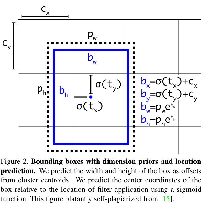
图中tx,ty是网络预测值,归一化0-1之间需要加sigmod,σ(tx),σ(ty)。所以这里gxy - gij就是制作的gt。后续和σ(tx),σ(ty)做ciou loss。
cx,cy就是gi,gj,就是单元格坐标!
这里是分别在缩放比例stridde=8,16,32上面的feature map上面整的,640大小的图的话对应的feature map大小是80,40,20.
制作好了gt,制作的gt主要是gxy - gij,gwh
当然这些信息同时附带了哪个单元格(gi,gj),哪个anchor,anchor对应的具体值,类别等信息。
tcls, tbox, indices, anch,为了后续计算对应的loss。
2. 计算loss部分 --中心点落在哪个单元格,该单元格就负责预测这个目标
        for i, pi in enumerate(p):  # layer index, layer predictions
            #pi [4,3,80,80,85]  [4,3,40,40,85]  [4,3,20,20,85]
            #tmp_0 = pi[..., 0] #[4,3,80,80]
            #b[95]  a[95]  gi[95]  gj[95]
            b, a, gj, gi = indices[i]  # image, anchor, gridy, gridx
            #tobj  [4,3,80,80]
            tobj = torch.zeros_like(pi[..., 0], device=device)  # target obj

            n = b.shape[0]  # number of targets
            if n:
                ## ps [95,85]
                ps = pi[b, a, gj, gi]  # prediction subset corresponding to targets
                # 这里需要仔细看下,这里pi是网络输出的值,
                # 而b,a,gj,gi都是目标gt的信息
                #所以这里就是为了让网络输出的值相应位置也要和gt一样!

                # Regression
                pxy = ps[:, :2].sigmoid() * 2. - 0.5  #[95,2]
                pwh = (ps[:, 2:4].sigmoid() * 2) ** 2 * anchors[i] #[95,2]
                pbox = torch.cat((pxy, pwh), 1)  # predicted box  #[95,4]
                '''
                pxy加sigmod是为了让值变为0-1之间数值,pxy是小数,就是相对于某个单元格是小数坐标。
                单元格是相应位置,已经根据gj,gi获取到了,ps = pi[b, a, gj, gi]
                就是代表着坐标【gi,gj】,你这个位置来负责和目标gt一样!

                pwh同样需要sigmod把值归一化到0-1之间,然后乘上anchors[i],因为anchor的长宽与gt相差不大了,就是4倍左右。
                所以把网络预测值×2再平方
                [0-1] --> [0,2] -->[0,4]  ||||  (ps[:, 2:4].sigmoid() * 2) ** 2
                '''
                iou = bbox_iou(pbox.T, tbox[i], x1y1x2y2=False, CIoU=True)  # iou(prediction, target)  [95]
                lbox += (1.0 - iou).mean()  # iou loss  [1]
这里有一处很重要,网络预测出来的尺寸之一是pi [4,3,80,80,85],80,80是640下采样8倍,85其中80是类别信息,x,y,w,h,is_obj再加上这5类。3是因为anchor里面有3个不同长宽比的尺寸。4是batchsize。
看上面代码一开始看不出哪里体现了 “中心点落在哪个单元格,该单元格就负责预测这个目标”。 其实下面这句话就是:
ps = pi[b, a, gj, gi]
pi的shape[4,3,80,80,85],
b, a, gj, gi是通过函数build_targets获取的,就是制作的gt,
a是具体哪个anchor,gi,gj是哪个单元格。
#b[95] a[95] gi[95] gj[95] ##3个缩放尺寸上总共匹配了95个目标gt
b, a, gj, gi里面的值都是当前范围内的索引!
ps = pi[b, a, gj, gi]这句话意思就是从pi对应位置取出!
所以得到的ps的shape是[95,85]。
这样就体现了 “中心点落在哪个单元格,该单元格就负责预测这个目标”。
然后后续就直接预测偏移量,和哪个单元格没有关系了。因为本身取出的值就是从网络输出的那个单元格取出的。
然后后续就是计算ciou,is_obj,class这三个loss。
哎呀,我是不是太唠叨了,所有的代码注释都有。
还不够精简,这里再精简总结一下流程:
step_1. gt与anchor绑定
1.1 在3个缩放系数8,16,32的gt下面,每个gt与每个anchor(总共3个)长宽差不多的gt保留。
1.2 保存在3个缩放系数下gt与anchor差不多的gt的信息,gi,gj,cls,a,anch等信息
step_2. 在网路预测的pi根据gi,gj,cls,a,anch同样取出相应位置上面的值计算ciou loss
step_3. 计算loss_is_obj, 每个边界框都预测了一个分数 objectness score,打分依据是预测框与物体的重叠度。
step_4. 计算loss_class