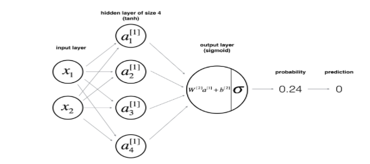
1、本次搭建的神经网络模型具有一个隐藏层的二分类
2、需要的激活函数有tanh,sigmoid
3、用了正向传播和反向传播。
4、计算交叉熵损失。
模型如下:
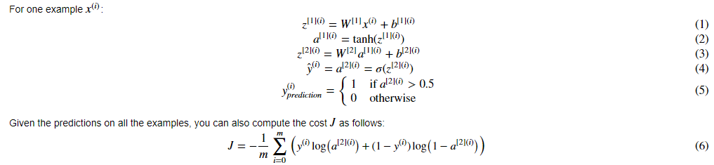
用到的数学公式:
建立神经网络的一般方法是:
1、定义神经网络结构(比如输入单元、隐藏单元等等)
2、初始化模型的参数
3、循环(迭代次数):
⑴实现向前传播
⑵计算损失
⑶实现向后传播以获得渐变
⑷更新参数(梯度下降)
1、定义神经网络结构
本次设置隐藏层大小为4
n_x:输入层的大小。
n_h:隐藏层的大小(将其设置为4)
n_y:输出层的大小。


 1 def layer_sizes(X, Y):
 2     """
 3     Arguments:
 4     X -- input dataset of shape (input size, number of examples)
 5     Y -- labels of shape (output size, number of examples)
 6
 7     Returns:
 8     n_x -- the size of the input layer
 9     n_h -- the size of the hidden layer
10     n_y -- the size of the output layer
11     """
12     ### START CODE HERE ### (≈ 3 lines of code)
13     n_x = X.shape[0] # size of input layer
14     n_h = 4
15     n_y = Y.shape[0] # size of output layer
16     ### END CODE HERE ###
17     return (n_x, n_h, n_y)
2、初始化模型的参数
使用随机值初始化权重矩阵、将偏差向量初始化为零。
 1 def initialize_parameters(n_x, n_h, n_y):
 2     """
 3     Argument:
 4     n_x -- size of the input layer
 5     n_h -- size of the hidden layer
 6     n_y -- size of the output layer
 7
 8     Returns:
 9     params -- python dictionary containing your parameters:
10                     W1 -- weight matrix of shape (n_h, n_x)
11                     b1 -- bias vector of shape (n_h, 1)
12                     W2 -- weight matrix of shape (n_y, n_h)
13                     b2 -- bias vector of shape (n_y, 1)
14     """
15
16     np.random.seed(2) # we set up a seed so that your output matches ours although the initialization is random.
17
18     ### START CODE HERE ### (≈ 4 lines of code)
19     W1 = np.random.randn(n_h, n_x) * 0.01
20     b1 = np.zeros((n_h, 1))
21     W2 = np.random.randn(n_y, n_h) * 0.01
22     b2 = np.zeros((n_y, 1))
23     ### END CODE HERE ###
24
25     assert (W1.shape == (n_h, n_x))
26     assert (b1.shape == (n_h, 1))
27     assert (W2.shape == (n_y, n_h))
28     assert (b2.shape == (n_y, 1))
29
30     parameters = {"W1": W1,
31                   "b1": b1,
32                   "W2": W2,
33                   "b2": b2}
34
35     return parameters
3、循环
⑴向前传播:
向前传播需要计算Z1、A1、Z2、A2,将计算得到的值存储在缓存里,方便反向传播的计算
激活函数用tanh和sigmoid。
 1 def forward_propagation(X, parameters):
 2     """
 3     Argument:
 4     X -- input data of size (n_x, m)
 5     parameters -- python dictionary containing your parameters (output of initialization function)
 6
 7     Returns:
 8     A2 -- The sigmoid output of the second activation
 9     cache -- a dictionary containing "Z1", "A1", "Z2" and "A2"
10     """
11     # Retrieve each parameter from the dictionary "parameters"
12     ### START CODE HERE ### (≈ 4 lines of code)
13     W1 = parameters['W1']
14     b1 = parameters['b1']
15     W2 = parameters['W2']
16     b2 = parameters['b2']
17     ### END CODE HERE ###
18
19     # Implement Forward Propagation to calculate A2 (probabilities)
20     ### START CODE HERE ### (≈ 4 lines of code)
21     Z1 = np.dot(W1,X)+b1
22     #A1 = sigmoid(Z1)
23     A1 = np.tanh(Z1)
24     Z2 = np.dot(W2,A1)+b2
25     #A2 = sigmoid(Z2)
26     A2 = sigmoid(Z2)
27     ### END CODE HERE ###
28
29     assert(A2.shape == (1, X.shape[1]))
30
31     cache = {"Z1": Z1,
32              "A1": A1,
33              "Z2": Z2,
34              "A2": A2}
35
36     return A2, cache
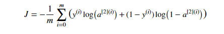
⑵计算代价成本 J
J的计算如下:
 1 def compute_cost(A2, Y, parameters):
 2     """
 3     Computes the cross-entropy cost given in equation (13)
 4
 5     Arguments:
 6     A2 -- The sigmoid output of the second activation, of shape (1, number of examples)
 7     Y -- "true" labels vector of shape (1, number of examples)
 8     parameters -- python dictionary containing your parameters W1, b1, W2 and b2
 9
10     Returns:
11     cost -- cross-entropy cost given equation (13)
12     """
13
14     m = Y.shape[1] # number of example
15
16     # Compute the cross-entropy cost
17     ### START CODE HERE ### (≈ 2 lines of code)
18     logprobs = np.multiply(np.log(A2),Y)+np.multiply((1-Y),np.log(1-A2))
19     cost = -1/m*np.sum(logprobs)
20     ### END CODE HERE ###
21
22     cost = np.squeeze(cost)     # makes sure cost is the dimension we expect.
23                                 # E.g., turns [[17]] into 17
24     assert(isinstance(cost, float))
25
26     return cost
⑶反向传播
用到的公式:
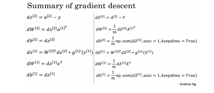
计算dZ1时需要用到g[1]'(Z[1]),由于激活函数是tanh,g(z)' = 1 − (g(z))2 ,即 g[1]'(Z[1]) = 1 - (g[1](Z[1]))2 。
当然,如果激活函数是sigmoid时,就是g(z)' = g(z)(1 − g(z))。
 1 def backward_propagation(parameters, cache, X, Y):
 2     """
 3     Implement the backward propagation using the instructions above.
 4
 5     Arguments:
 6     parameters -- python dictionary containing our parameters
 7     cache -- a dictionary containing "Z1", "A1", "Z2" and "A2".
 8     X -- input data of shape (2, number of examples)
 9     Y -- "true" labels vector of shape (1, number of examples)
10
11     Returns:
12     grads -- python dictionary containing your gradients with respect to different parameters
13     """
14     m = X.shape[1]
15
16     # First, retrieve W1 and W2 from the dictionary "parameters".
17     ### START CODE HERE ### (≈ 2 lines of code)
18     W1 = parameters['W1']
19     W2 = parameters['W2']
20     ### END CODE HERE ###
21
22     # Retrieve also A1 and A2 from dictionary "cache".
23     ### START CODE HERE ### (≈ 2 lines of code)
24     A1 = cache['A1']
25     A2 = cache['A2']
26     ### END CODE HERE ###
27
28     # Backward propagation: calculate dW1, db1, dW2, db2.
29     ### START CODE HERE ### (≈ 6 lines of code, corresponding to 6 equations on slide above)
30     dZ2 = A2-Y
31     dW2 = 1/m*np.dot(dZ2,A1.T)
32     db2 = 1/m*np.sum(dZ2,axis=1,keepdims=True)
33     dZ1 = np.dot(W2.T,dZ2)*(1 - np.power(A1, 2))
34     dW1 = 1/m*np.dot(dZ1,X.T)
35     db1 = 1/m*np.sum(dZ1,axis=1,keepdims=True)
36     ### END CODE HERE ###
37
38     grads = {"dW1": dW1,
39              "db1": db1,
40              "dW2": dW2,
41              "db2": db2}
42
43     return grads
⑷更新参数
通过 更新参数。
更新参数。
 1 def update_parameters(parameters, grads, learning_rate = 1.2):
 2     """
 3     Updates parameters using the gradient descent update rule given above
 4
 5     Arguments:
 6     parameters -- python dictionary containing your parameters
 7     grads -- python dictionary containing your gradients
 8
 9     Returns:
10     parameters -- python dictionary containing your updated parameters
11     """
12     # Retrieve each parameter from the dictionary "parameters"
13     ### START CODE HERE ### (≈ 4 lines of code)
14     W1 = parameters['W1']
15     b1 = parameters['b1']
16     W2 = parameters['W2']
17     b2 = parameters['b2']
18     ### END CODE HERE ###
19
20     # Retrieve each gradient from the dictionary "grads"
21     ### START CODE HERE ### (≈ 4 lines of code)
22     dW1 = grads['dW1']
23     db1 = grads['db1']
24     dW2 = grads['dW2']
25     db2 = grads['db2']
26     ## END CODE HERE ###
27
28     # Update rule for each parameter
29     ### START CODE HERE ### (≈ 4 lines of code)
30     W1 -= learning_rate*dW1
31     b1 -= learning_rate*db1
32     W2 -= learning_rate*dW2
33     b2 -= learning_rate*db2
34     ### END CODE HERE ###
35
36     parameters = {"W1": W1,
37                   "b1": b1,
38                   "W2": W2,
39                   "b2": b2}
40
41     return parameters
4、将之前的合并到一个函数里
 1 def nn_model(X, Y, n_h, num_iterations = 10000, print_cost=False):
 2     """
 3     Arguments:
 4     X -- dataset of shape (2, number of examples)
 5     Y -- labels of shape (1, number of examples)
 6     n_h -- size of the hidden layer
 7     num_iterations -- Number of iterations in gradient descent loop
 8     print_cost -- if True, print the cost every 1000 iterations
 9
10     Returns:
11     parameters -- parameters learnt by the model. They can then be used to predict.
12     """
13
14     np.random.seed(3)
15     n_x = layer_sizes(X, Y)[0]
16     n_y = layer_sizes(X, Y)[2]
17
18     # Initialize parameters, then retrieve W1, b1, W2, b2. Inputs: "n_x, n_h, n_y". Outputs = "W1, b1, W2, b2, parameters".
19     ### START CODE HERE ### (≈ 5 lines of code)
20     parameters = initialize_parameters(n_x, n_h, n_y)
21     W1 = parameters['W1']
22     b1 = parameters['b1']
23     W2 = parameters['W2']
24     b2 = parameters['b2']
25     ### END CODE HERE ###
26
27     # Loop (gradient descent)
28
29     for i in range(0, num_iterations):
30
31         ### START CODE HERE ### (≈ 4 lines of code)
32         # Forward propagation. Inputs: "X, parameters". Outputs: "A2, cache".
33         A2, cache = forward_propagation(X, parameters)
34
35         # Cost function. Inputs: "A2, Y, parameters". Outputs: "cost".
36         cost = compute_cost(A2, Y, parameters)
37
38         # Backpropagation. Inputs: "parameters, cache, X, Y". Outputs: "grads".
39         grads = backward_propagation(parameters, cache, X, Y)
40
41         # Gradient descent parameter update. Inputs: "parameters, grads". Outputs: "parameters".
42         parameters = update_parameters(parameters, grads)
43
44         ### END CODE HERE ###
45
46         # Print the cost every 1000 iterations
47         if print_cost and i % 1000 == 0:
48             print ("Cost after iteration %i: %f" %(i, cost))
49
50     return parameters
5、预测
可以写一个预测函数,用来验证得到的神经网络模型的效果怎么样。
预测使用下面规则:
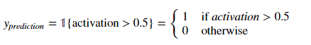
 1 def predict(parameters, X):
 2     """
 3     Using the learned parameters, predicts a class for each example in X
 4
 5     Arguments:
 6     parameters -- python dictionary containing your parameters
 7     X -- input data of size (n_x, m)
 8
 9     Returns
10     predictions -- vector of predictions of our model (red: 0 / blue: 1)
11     """
12
13     # Computes probabilities using forward propagation, and classifies to 0/1 using 0.5 as the threshold.
14     ### START CODE HERE ### (≈ 2 lines of code)
15     A2, cache = forward_propagation(X, parameters)
16     predictions = (A2 > 0.5)
17     ### END CODE HERE ###
18
19     return predictions
6、其它
由于nn_model模型已经封装好了,现在只需要传入参数就可以得到结果了。然后我们可以调参,设置不同的隐藏层大小来得到不同的效果,依次选择最佳的值。
plt.figure(figsize=(16, 32))
hidden_layer_sizes = [1, 2, 3, 4, 5, 20, 50]
for i, n_h in enumerate(hidden_layer_sizes):
    plt.subplot(5, 2, i+1)
    plt.title('Hidden Layer of size %d' % n_h)
    parameters = nn_model(X, Y, n_h, num_iterations = 5000)
    plot_decision_boundary(lambda x: predict(parameters, x.T), X, Y)
    predictions = predict(parameters, X)
    accuracy = float((np.dot(Y,predictions.T) + np.dot(1-Y,1-predictions.T))/float(Y.size)*100)
    print ("Accuracy for {} hidden units: {} %".format(n_h, accuracy))
得到的准确率如下:
Accuracy for 1 hidden units: 67.5 %
Accuracy for 2 hidden units: 67.25 %
Accuracy for 3 hidden units: 90.75 %
Accuracy for 4 hidden units: 90.5 %
Accuracy for 5 hidden units: 91.25 %
Accuracy for 20 hidden units: 90.0 %
Accuracy for 50 hidden units: 90.25 %
可以看到隐藏层大小为5时效果最佳,可见不是越大越好,也不是越小越好。根据不同的问题需要选择不同的值。