参考博客:http://www.360doc.com/content/17/1123/17/35874779_706497143.shtml
XGBoost参数详解
在运行XGboost之前,必须设置三种类型成熟:general parameters,booster parameters和task parameters:
General parameters 该参数参数控制在提升(boosting)过程中使用哪种booster,常用的booster有树模型(tree)和线性模型(linear model)
Booster parameters 这取决于使用哪种booster
Task parameters 控制学习的场景,例如在回归问题中会使用不同的参数控制排序
1)General Parameters
booster [default=gbtree]
有两种模型可以选择gbtree和gblinear。gbtree使用基于树的模型进行提升计算,gblinear使用线性模型进行提升计算。缺省值为gbtree。
silent [default=0]
取0时表示打印出运行时信息,取1时表示以缄默方式运行,不打印运行时信息。缺省值为0。
nthread
XGBoost运行时的线程数。缺省值是当前系统可以获得的最大线程数。
num_pbuffer
预测缓冲区大小,通常设置为训练实例的数目。缓冲用于保存最后一步提升的预测结果,无需人为设置。
num_feature
Boosting过程中用到的特征维数,设置为特征个数。XGBoost会自动设置,无需人为设置。
2)Parameters for Tree Booster
eta [default=0.3]
为了防止过拟合,更新过程中用到的收缩步长。在每次提升计算之后,算法会直接获得新特征的权重。 eta通过缩减特征的权重使提升计算过程更加保守。缺省值为0.3 。取值范围为:[0,1]
gamma [default=0]
minimum loss reduction required to make a further partition on a leaf node of the tree. the larger, the more conservative the algorithm will be. 取值范围为:[0,∞]
max_depth [default=6]
数的最大深度。缺省值为6。取值范围为:[1,∞]
min_child_weight [default=1]
孩子节点中最小的样本权重和。如果一个叶子节点的样本权重和小于min_child_weight则拆分过程结束。在现行回归模型中,这个参数是指建立每个模型所需要的最小样本数。该成熟越大算法越conservative。取值范围为:[0,∞]
max_delta_step [default=0]
我们允许每个树的权重被估计的值。如果它的值被设置为0,意味着没有约束;如果它被设置为一个正值,它能够使得更新的步骤更加保守。通常这个参数是没有必要的,但是如果在逻辑回归中类极其不平衡这时候他有可能会起到帮助作用。把它范围设置为1-10之间也许能控制更新。 取值范围为:[0,∞]
subsample [default=1]
用于训练模型的子样本占整个样本集合的比例。如果设置为0.5则意味着XGBoost将随机的从整个样本集合中随机的抽取出50%的子样本建立树模型,这能够防止过拟合。 取值范围为:(0,1]
colsample_bytree [default=1]
在建立树时对特征采样的比例。缺省值为1。取值范围为:(0,1]
3) Parameter for Linear Booster
lambda [default=0]
L2 正则的惩罚系数
alpha [default=0]
L1 正则的惩罚系数
lambda_bias
在偏置上的L2正则。缺省值为0(在L1上没有偏置项的正则,因为L1时偏置不重要)。
4)Task Parameters
objective [ default=reg:linear ]
定义学习任务及相应的学习目标,可选的目标函数如下:
“reg:linear” —— 线性回归。
“reg:logistic”—— 逻辑回归。
“binary:logistic”—— 二分类的逻辑回归问题,输出为概率。
“binary:logitraw”—— 二分类的逻辑回归问题,输出的结果为wTx。
“count:poisson”—— 计数问题的poisson回归,输出结果为poisson分布。在poisson回归中,max_delta_step的缺省值为0.7。(used to safeguard optimization)
“multi:softmax” –让XGBoost采用softmax目标函数处理多分类问题,同时需要设置参数num_class(类别个数)
“multi:softprob” –和softmax一样,但是输出的是ndata * nclass的向量,可以将该向量reshape成ndata行nclass列的矩阵。没行数据表示样本所属于每个类别的概率。
“rank:pairwise” –set XGBoost to do ranking task by minimizing the pairwise loss。
base_score [ default=0.5 ]
所有实例的初始化预测分数,全局偏置;为了足够的迭代次数,改变这个值将不会有太大的影响。
eval_metric [ default according to objective ]
校验数据所需要的评价指标,不同的目标函数将会有缺省的评价指标(rmse for regression, and error for classification, mean average precision for ranking)。
用户可以添加多种评价指标,对于Python用户要以list传递参数对给程序,而不是map参数list参数不会覆盖’eval_metric’。
可供的选择如下:
“rmse”: root mean square error
“logloss”: negative log-likelihood
“error”: Binary classification error rate. It is calculated as #(wrong cases)/#(all cases). For the predictions, the evaluation will regard the instances with prediction value larger than 0.5 as positive instances, and the others as negative instances.
“merror”: Multiclass classification error rate.
“mlogloss”: Multiclass logloss.
“auc”: Area under the curve for ranking evaluation.
“ndcg”:Normalized Discounted Cumulative Gain
“map”:Mean average precision
“ndcg@n”,”map@n”: n can be assigned as an integer to cut off the top positions in the lists for evaluation.
“ndcg-“,”map-“,”ndcg@n-“,”map@n-“: In XGBoost, NDCG andMAP will evaluate the score of a list without any positive samples as 1. By adding “-” in the evaluation metric XGBoostwill evaluate these score as 0 to be consistent under some conditions. training repeatively
seed [ default=0 ]
随机数的种子。缺省值为0。
XGBoost 实战
XGBoost有两大类接口:XGBoost原生接口 和 scikit-learn接口 ,并且XGBoost能够实现 分类 和 回归 两种任务。因此,本章节分四个小块来介绍!
1、基于XGBoost原生接口的分类
from sklearn.datasets import load_iris
import xgboost as xgb
from xgboost import plot_importance
from matplotlib import pyplot as plt
from sklearn.model_selection import train_test_split
# read in the iris data
iris = load_iris()
X = iris.data
y = iris.target
X_train, X_test, y_train, y_test = train_test_split(X, y, test_size=0.2, random_state=1234565)
params = {
'booster': 'gbtree',
'objective': 'multi:softmax',
'num_class': 3,
'gamma': 0.1,
'max_depth': 6,
'lambda': 2,
'subsample': 0.7,
'colsample_bytree': 0.7,
'min_child_weight': 3,
'silent': 1,
'eta': 0.1,
'seed': 1000,
'nthread': 4,
}
plst = params.items()
dtrain = xgb.DMatrix(X_train, y_train)
num_rounds = 500
model = xgb.train(plst, dtrain, num_rounds)
# 对测试集进行预测
dtest = xgb.DMatrix(X_test)
ans = model.predict(dtest)
# 计算准确率
cnt1 = 0
cnt2 = 0
for i in range(len(y_test)):
if ans[i] == y_test[i]:
cnt1 += 1
else:
cnt2 += 1
print('Accuracy: %.2f %% ' % (100 * cnt1 / (cnt1 + cnt2)))
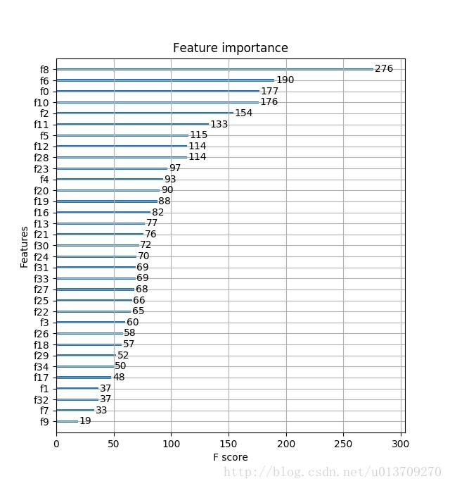
# 显示重要特征
plot_importance(model)
plt.show()

2、基于XGBoost原生接口的回归
import xgboost as xgb
from xgboost import plot_importance
from matplotlib import pyplot as plt
from sklearn.model_selection import train_test_split

# 读取文件原始数据
data = []
labels = []
labels2 = []
with open('lppz5.csv', encoding='UTF-8') as fileObject:
   for line in fileObject:
       line_split = line.split(',')
       data.append(line_split[10:])
       labels.append(line_split[8])

X = []
for row in data:
   row = [float(x) for x in row]
   X.append(row)

y = [float(x) for x in labels]

# XGBoost训练过程
X_train, X_test, y_train, y_test = train_test_split(X, y, test_size=0.2, random_state=0)

params = {
   'booster': 'gbtree',
   'objective': 'reg:gamma',
   'gamma': 0.1,
   'max_depth': 5,
   'lambda': 3,
   'subsample': 0.7,
   'colsample_bytree': 0.7,
   'min_child_weight': 3,
   'silent': 1,
   'eta': 0.1,
   'seed': 1000,
   'nthread': 4,
}

dtrain = xgb.DMatrix(X_train, y_train)
num_rounds = 300
plst = params.items()
model = xgb.train(plst, dtrain, num_rounds)

# 对测试集进行预测
dtest = xgb.DMatrix(X_test)
ans = model.predict(dtest)

# 显示重要特征
plot_importance(model)
plt.show()

3、基于Scikit-learn接口的分类
from sklearn.datasets import load_iris
import xgboost as xgb
from xgboost import plot_importance
from matplotlib import pyplot as plt
from sklearn.model_selection import train_test_split

# read in the iris data
iris = load_iris()

X = iris.data
y = iris.target

X_train, X_test, y_train, y_test = train_test_split(X, y, test_size=0.2, random_state=0)

# 训练模型
model = xgb.XGBClassifier(max_depth=5, learning_rate=0.1, n_estimators=160, silent=True, objective='multi:softmax')
model.fit(X_train, y_train)

# 对测试集进行预测
ans = model.predict(X_test)

# 计算准确率
cnt1 = 0
cnt2 = 0
for i in range(len(y_test)):
   if ans[i] == y_test[i]:
       cnt1 += 1
   else:
       cnt2 += 1

print('Accuracy: %.2f %% ' % (100 * cnt1 / (cnt1 + cnt2)))

# 显示重要特征
plot_importance(model)
plt.show()

4)基于XGBoost原生接口的回归
import xgboost as xgb
from xgboost import plot_importance
from matplotlib import pyplot as plt
from sklearn.model_selection import train_test_split

# 读取文件原始数据
data = []
labels = []
labels2 = []
with open('lppz5.csv', encoding='UTF-8') as fileObject:
   for line in fileObject:
       line_split = line.split(',')
       data.append(line_split[10:])
       labels.append(line_split[8])

X = []
for row in data:
   row = [float(x) for x in row]
   X.append(row)

y = [float(x) for x in labels]

# XGBoost训练过程
X_train, X_test, y_train, y_test = train_test_split(X, y, test_size=0.2, random_state=0)

model = xgb.XGBRegressor(max_depth=5, learning_rate=0.1, n_estimators=160, silent=True, objective='reg:gamma')
model.fit(X_train, y_train)

# 对测试集进行预测
ans = model.predict(X_test)

# 显示重要特征
plot_importance(model)
plt.show()