【论文翻译】NIN层论文中英对照翻译--（Network In Network）

【开始时间】2018.09.27

【完成时间】2018.10.03

【中文译名】网络中的网络

【补充】

1）NIN结构的caffe实现：

因为我们可以把全连接层当作为特殊的卷积层，所以呢， NIN在caffe中是非常容易实现的：

https://github.com/BVLC/caffe/wiki/Model-Zoo#network-in-network-model

这是由BVLC（Berkeley Vision Learning Center）维护的一个caffe的各种model及训练好的参数权值，可以直接下载下来用的；

2)NIN的第一个N指mlpconv,第二个N指整个深度网络结构，即整个深度网络是由多个mlpconv构成的。

3）论文的发表时间是： 4 Mar 2014

题目：网络中的网络

Abstract（摘要）

We propose a novel deep network structure called “Network In Network”(NIN) to enhance model discriminability for local patches within the receptive field. The conventional convolutional layer uses linear filters followed by a nonlinear activation function to scan the input. Instead, we build micro neural networks with more complex structures to abstract the data within the receptive field. We instantiate the micro neural network with a multilayer perceptron, which is a potent function approximator. The feature maps are obtained by sliding the micro networks over the input in a similar manner as CNN; they are then fed into the next layer. Deep NIN can be implemented by stacking mutiple of the above described structure. With enhanced local modeling via the micro network, we are able to utilize global average pooling over feature maps in the classification layer, which is easier to interpret and less prone to overfitting than traditional fully connected layers. We demonstrated the state-of-the-art classification performances with NIN on CIFAR-10 and CIFAR-100, and reasonable performances on SVHN and MNIST datasets.

我们提出了一种新的深层网络结构-“网络中的网络”(NetworkinNetwork，nin)，以提高接收域内局部区域的模型识别能力。传统的卷积层采用线性滤波器和非线性增益函数对输入进行扫描。作为替代的，我们建立了具有更复杂结构的微神经网络来抽象接受域内的数据。我们用一个多层感知器实例化了微型神经网络，它是一种强有效的函数逼近器。特征映射是通过将微网络以类似于CNN的方式在输入上滑动获得的，然后将它们输入到下一层。通过上述结构的多层叠加，可以实现深度nin。通过微网络增强局部建模，我们能够在分类层对特征图进行全局平均池化，这比传统的完全连接的图层更容易解释，也不太容易过拟合。我们展示了NIN在CIFAR-10和CIFAR-100上得到了有史以来最佳的表现以及在SVHN和MNIST数据集上合理的表现。

1 Introduction（介绍）

Convolutional neural networks (CNNs) [1] consist of alternating convolutional layers and pooling layers. Convolution layers take inner product of the linear filter and the underlying receptive field followed by a nonlinear activation function at every local portion of the input. The resulting outputs are called feature maps.

卷积神经网络(CNNs)[1]由交替的卷积层和汇聚层组成。卷积层在输入的每个局部部分取线性滤波器和底层接收场的内积，然后是一个非线性激活函数。结果输出称为特征映射。

The convolution filter in CNN is a generalized linear model (GLM) for the underlying data patch,and we argue that the level of abstraction is low with GLM. By abstraction we mean that the feature is invariant to the variants of the same concept [2]. Replacing the GLM with a more potent nonlinear function approximator can enhance the abstraction ability of the local model. GLM can achieve a good extent of abstraction when the samples of the latent concepts are linearly separable,i.e. the variants of the concepts all live on one side of the separation plane defined by the GLM. Thus conventional CNN implicitly makes the assumption that the latent concepts are linearly separable. However, the data for the same concept often live on a nonlinear manifold, therefore the representations that capture these concepts are generally highly nonlinear function of the input. In NIN, the GLM is replaced with a ”micro network” structure which is a general nonlinear function approximator. In this work, we choose multilayer perceptron [3] as the instantiation of the micro network,which is a universal function approximator and a neural network trainable by back-propagation.

CNN的卷积滤波器是底层数据块的广义线性模型（generalized linear model ）（GLM），而且我们认为它的抽象程度较低。抽象是指特征对同一概念的变体是不变的[2]。用更强（有效）的非线性函数逼近器代替GLM，可以提高局部模型的抽象能力。当样本的隐含概念（latent concept）是线性可分时，GLM可以达到很好的抽象程度，例如：这些概念的变体都在GLM分割平面的同一边。因此，传统的CNN隐含地假设潜在的概念是线性可分的。然而，同一概念的数据通常是非线性流形的（nonlinear manifold），捕捉这些概念的表达通常都是输入的高维非线性函数。在NIN中，用一种一般非线性函数逼近器的“微网络结构”代替了GLM。在本文中，我们选择多层感知器[3]作为微网络的实例化，它是一种通用函数逼近器，是一个可通过反向传播进行训练的神经网络。

The resulting structure which we call an mlpconv layer is compared with CNN in Figure 1. Both the linear convolutional layer and the mlpconv layer map the local receptive field to an output feature vector. The mlpconv maps the input local patch to the output feature vector with a multilayer perceptron (MLP) consisting of multiple fully connected layers with nonlinear activation functions. The MLP is shared among all local receptive fields. The feature maps are obtained by sliding the MLP over the input in a similar manner as CNN and are then fed into the next layer. The overall structure of the NIN is the stacking of multiple mlpconv layers. It is called “Network In Network” (NIN) as we have micro networks (MLP), which are composing elements of the overall deep network, within mlpconv layers.

我们称之为mlpconv层的结果结构在图1中与CNN进行了比较。线性卷积层和mlpconv层都将局部接收场映射到输出特征向量。 mlpconv 层将局部块（ input local patch）的输入通过一个由全连接层和非线性激活函数组成的多层感知器（MLP）映射到了输出的特征向量。 MLP在所有局部感受野中共享。特征图通过用像CNN一样的方式在输入上滑动MLP得到，NIN的总体结构是一系列mplconv层的堆叠。它被称为“网络中的网络”(NIN)，因为我们有微型网络(MLP)，它在mlpconv层中构成整个深层网络的组成部分。

Instead of adopting the traditional fully connected layers for classification in CNN, we directly output the spatial average of the feature maps from the last mlpconv layer as the confidence of categories via a global average pooling layer, and then the resulting vector is fed into the softmax layer. In traditional CNN, it is difficult to interpret how the category level information from the objective cost layer is passed back to the previous convolution layer due to the fully connected layers which act as a black box in between. In contrast, global average pooling is more meaningful and interpretable as it enforces correspondance between feature maps and categories, which is made possible by a stronger local modeling using the micro network. Furthermore, the fully connected layers are prone to overfitting and heavily depend on dropout regularization [4] [5], while global average pooling is itself a structural regularizer, which natively prevents overfitting for the overall structure.

我们不采用在CNN中传统的完全连通层进行分类，而是通过全局平均池层（global average pooling layer）直接输出最后一个mlpconv层的特征映射的空间平均值作为类别的可信度，然后将得到的向量输入到Softmax层。在传统的CNN中，很难解释如何将来自分类层（objective cost layer）的分类信息传递回前一个卷积层，因为全连接层像一个黑盒一样。相反，全局平均池更有意义和可解释，因为它强制特征映射和类别之间的对应，这是通过使用微型网络进行更强的局部建模而实现的。此外，完全连接层容易过度拟合，严重依赖于Dropout正则化[4][5]，而全局平均池本身就是一个结构正则化，这在本质上防止了对整体结构的过度拟合。

2 Convolutional Neural Networks（卷积神经网络）

Classic convolutional neuron networks [1] consist of alternatively stacked convolutional layers and spatial pooling layers. The convolutional layers generate feature maps by linear convolutional filters followed by nonlinear activation functions (rectifier, sigmoid, tanh, etc.). Using the linear rectifier as an example, the feature map can be calculated as follows:

经典卷积神经元网络[1]由交替叠加的卷积层和空间汇聚层组成。卷积层通过线性卷积滤波器和非线性激活函数(整流器（rectifier）、Sigmoid、tanh等)生成特征映射。以线性整流器为例，可以按以下方式计算特征图：

Here (i,j) is the pixel index in the feature map, x ij stands for the input patch centered at location(i,j), and k is used to index the channels of the feature map.

这里的(i, j)是特征图像素的索引，xij代表以位置(i, j)为中心的输入块，k用来索引特征图的颜色通道。

This linear convolution is sufficient for abstraction when the instances of the latent concepts are linearly separable. However, representations that achieve good abstraction are generally highly non-linear functions of the input data. In conventional CNN, this might be compensated by utilizing an over-complete set of filters [6] to cover all variations of the latent concepts. Namely, individual linear filters can be learned to detect different variations of a same concept. However, having too many filters for a single concept imposes extra burden on the next layer, which needs to consider all combinations of variations from the previous layer [7]. As in CNN, filters from higher layers map to larger regions in the original input. It generates a higher level concept by combining the lower level concepts from the layer below. Therefore, we argue that it would be beneficial to do a better abstraction on each local patch, before combining them into higher level concepts.

当隐性概念（ the latent concepts ）的实例是线性可分的时，这种线性卷积就足以进行抽象。然而，实现良好抽象的表示通常是输入数据的高度非线性函数。在传统的CNN中，这可以通过利用一套完整的滤波器来弥补，覆盖所有隐含概念的变化。也就是说，可以学习独立的线性滤波器来检测同一概念的不同变化。然而，对单个概念有太多的过滤器会给下一层带来额外的负担，（因为）下一层需要考虑上一层的所有变化组合[7]。在CNN中，来自更高层的滤波器会映射到原始输入的更大区域。它通过结合下面层中的较低级别概念来生成更高级别的概念。因此，我们认为，在将每个本地块（local patch）合并为更高级别的概念之前，对每个本地快进行更好的抽象是有益的。

In the recent maxout network [8], the number of feature maps is reduced by maximum pooling over affine feature maps (affine feature maps are the direct results from linear convolution without applying the activation function). Maximization over linear functions makes a piecewise linear approximator which is capable of approximating any convex functions. Compared to conventional convolutional layers which perform linear separation, the maxout network is more potent as it can

separate concepts that lie within convex sets. This improvement endows the maxout network with the best performances on several benchmark datasets.

在最近的Maxout网络[8]中，特征映射的数目通过仿射特征映射上的最大池来减少(仿射特征映射是线性卷积不应用激活函数的直接结果)。线性函数的极大化使分段线性逼近器( piecewise linear approximator)能够逼近任意凸函数。与进行线性分离的传统卷积层相比，最大输出网络更强大，因为它能够分离凸集中的概念。这种改进使maxout网络在几个基准数据集上有最好的表现。

However, maxout network imposes the prior that instances of a latent concept lie within a convex set in the input space, which does not necessarily hold. It would be necessary to employ a more general function approximator when the distributions of the latent concepts are more complex. We seek to achieve this by introducing the novel “Network In Network” structure, in which a micro network is introduced within each convolutional layer to compute more abstract features for local patches.

但是，Maxout网络强制要求潜在概念的实例存在于输入空间中的凸集中，这并不一定成立。当隐性概念的分布更加复杂时，需要使用更一般的函数逼近器。我们试图通过引入一种新颖的“Network In Network”结构来实现这一目标，即在每个卷积层中引入一个微网络来计算局部块的更抽象的特征。

Sliding a micro network over the input has been proposed in several previous works. For example, the Structured Multilayer Perceptron (SMLP) [9] applies a shared multilayer perceptron on different patches of the input image; in another work, a neural network based filter is trained for face detection[10]. However, they are both designed for specific problems and both contain only one layer of the sliding network structure. NIN is proposed from a more general perspective, the micro network is integrated into CNN structure in persuit of better abstractions for all levels of features.

在以前的一些工作中，已经提出了在输入端滑动一个微网络。例如，结构化多层感知器(SMLP)[9]在输入图像的不同块上应用共享多层感知器；在另一项工作中，基于神经网络的滤波器被训练用于人脸检测[10]。然而，它们都是针对特定的问题而设计的，而且都只包含一层滑动网络结构。NIN是从更一般的角度提出的，将微网络集成到CNN结构中，对各个层次的特征进行更好的抽象。

3 Network In Network（网络中的网络）

We first highlight the key components of our proposed “Network In Network” structure: the MLP convolutional layer and the global averaging pooling layer in Sec. 3.1 and Sec. 3.2 respectively.Then we detail the overall NIN in Sec. 3.3.

我们首先强调了我们提出的“网络中的网络”结构的关键组成部分：MLP卷积层和全局平均池层分别在3.1节和3.2节中。然后我们在3.3节中详细描述整个nin。

3.1 MLP Convolution Layers（MLP卷积层）

Given no priors about the distributions of the latent concepts, it is desirable to use a universal function approximator for feature extraction of the local patches, as it is capable of approximating more abstract representations of the latent concepts. Radial basis network and multilayer perceptron are two well known universal function approximators. We choose multilayer perceptron in this work for two reasons. First, multilayer perceptron is compatible with the structure of convolutional neural networks, which is trained using back-propagation. Second, multilayer perceptron can be a deep model itself, which is consistent with the spirit of feature re-use [2]. This new type of layer is called mlpconv in this paper, in which MLP replaces the GLM to convolve over the input. Figure1 illustrates the difference between linear convolutional layer and mlpconv layer. The calculation performed by mlpconv layer is shown as follows:

由于没有关于潜在概念分布的先验信息，使用通用函数逼近器来提取局部块的特征是可取的，因为它能够逼近潜在概念的更抽象的表示。径向基网络和多层感知器是两种著名的通用函数逼近器。我们在这项工作中选择多层感知器有两个原因。首先，多层感知器与采用反向传播训练的卷积神经网络的结构兼容；第二，多层感知器本身可以是一个深层次的模型，这与特征重用的精神是一致的[2]。在本文中，这种新型的层称为mlpconv，其中MLP取代GLM，在输入上进行转换。图1说明了线性卷积层和mlpconv层之间的区别。由mlpconv层执行的计算如下：

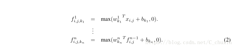
Here n is the number of layers in the multilayer perceptron. Rectified linear unit is used as the activation function in the multilayer perceptron.

这里n是多层感知器中的层数。在多层感知器中，采用整流线性单元作为激活函数。

图1、线性卷积层与mlpconv层的比较。线性卷积层包括线性滤波器，而mlpconv层包含微网络(本文选择了多层感知器)。这两层都将局部接受域映射为隐性概念的置信度值。

From cross channel (cross feature map) pooling point of view, Equation 2 is equivalent to cascaded cross channel parametric pooling on a normal convolution layer. Each pooling layer performs weighted linear recombination on the input feature maps, which then go through a rectifier linear unit. The cross channel pooled feature maps are cross channel pooled again and again in the next layers. This cascaded cross channel parameteric pooling structure allows complex and learnable interactions of cross channel information.

从跨信道(跨特征图--cross feature map)池的角度看，方程2等价于正规卷积层上的级联跨信道参数池( cascaded cross channel parametric pooling)。每个池层对输入特征映射执行加权线性重组，然后通过整流线性单元。跨通道池功能映射在下一层中一次又一次地跨通道池。这种级联的跨信道参数池结构允许复杂且可学习的交叉信道信息交互。

The cross channel parametric pooling layer is also equivalent to a convolution layer with 1x1 convolution kernel. This interpretation makes it straightforawrd to understand the structure of NIN.

跨信道参数池层也等价于具有1x1卷积核的卷积层。这一解释使得理解nin的结构更为直观。

Comparison to maxout layers: the maxout layers in the maxout network performs max pooling across multiple affine feature maps [8]. The feature maps of maxout layers are calculated as follows:

与maxout层的比较：maxout网络中的maxout层跨多个仿射特征映射执行max池化[8]。最大层的特征图计算如下：

Maxout over linear functions forms a piecewise linear function which is capable of modeling any convex function. For a convex function, samples with function values below a specific threshold form a convex set. Therefore, by approximating convex functions of the local patch, maxout has the capability of forming separation hyperplanes for concepts whose samples are within a convex set (i.e. l 2 balls, convex cones). Mlpconv layer differs from maxout layer in that the convex function approximator is replaced by a universal function approximator, which has greater capability in modeling various distributions of latent concepts.

线性函数上的极大值形成一个分段线性函数，它能够建模任何凸函数。对于凸函数，函数值低于特定阈值的样本构成凸集。因此，通过逼近局部块的凸函数，maxout对样本位于凸集(即L2球、凸锥)的概念具有形成分离超平面的能力。mlpconv层与maxout层的不同之处在于，凸函数逼近器被一个通用函数逼近器所代替，它在建模各种隐性概念分布方面具有更强的能力。

3.2 Global Average Pooling（全球平均池化）

Conventional convolutional neural networks perform convolution in the lower layers of the network.For classification, the feature maps of the last convolutional layer are vectorized and fed into fully connected layers followed by a softmax logistic regression layer [4] [8] [11]. This structure bridges the convolutional structure with traditional neural network classifiers. It treats the convolutional layers as feature extractors, and the resulting feature is classified in a traditional way.

传统的卷积神经网络在网络的底层进行卷积。在分类方面，将上一卷积层的特征映射矢量化，并将其输入到完全连通的层中，然后是Softmax Logistic回归层[4][8][11]。该结构将卷积结构与传统的神经网络分类器连接起来。它将卷积层作为特征提取器，并对生成的特征进行传统的分类。

However, the fully connected layers are prone to overfitting, thus hampering the generalization ability of the overall network. Dropout is proposed by Hinton et al. [5] as a regularizer which randomly sets half of the activations to the fully connected layers to zero during training. It has improved the generalization ability and largely prevents overfitting [4].

然而，全连通层容易过度拟合，从而阻碍了整个网络的泛化能力。Dropout是由Hinton等人提出的[5]。它作为一个正则化，在训练期间随机地将半个完全连接的层的激活设置为零。它提高了泛化能力，在很大程度上防止了过度拟合[4]。

In this paper, we propose another strategy called global average pooling to replace the traditional fully connected layers in CNN. The idea is to generate one feature map for each corresponding category of the classification task in the last mlpconv layer. Instead of adding fully connected layers on top of the feature maps, we take the average of each feature map, and the resulting vector is fed directly into the softmax layer. One advantage of global average pooling over the fully connected layers is that it is more native to the convolution structure by enforcing correspondences between feature maps and categories.Thus the feature maps can be easily interpreted as categories confidence maps. Another advantage is that there is no parameter to optimize in the global average pooling thus overfitting is avoided at this layer. Futhermore, global average pooling sums out the spatial information, thus it is more robust to spatial translations of the input.

在本文中，我们提出了另一种策略，称为全局平均池，以取代CNN中传统的全连通层。其思想是为最后一个mlpconv层中的分类任务的每个对应类别生成一个特征映射。我们没有在特征映射的顶部添加完全连通的层，而是取每个特征映射的平均值，并将得到的向量直接输入到Softmax层。全局平均池取代完全连通层上的一个优点是，通过增强特征映射和类别之间的对应关系，它更适合于卷积结构。因此，特征映射可以很容易地解释为类别信任映射。另一个优点是在全局平均池中没有优化参数，从而避免了这一层的过度拟合。此外，全局平均池综合了空间信息，从而对输入的空间平移具有更强的鲁棒性。

We can see global average pooling as a structural regularizer that explicitly enforces feature maps to be confidence maps of concepts (categories). This is made possible by the mlpconv layers, as they makes better approximation to the confidence maps than GLMs.

我们可以看到全局平均池是一个结构正则化器，它显式地将特征映射强制为概念(类别)的信任映射。这是由mlpconv层实现的，因为它们比GLMS更接近置信度图。

3.3 Network In Network Structure（网络的网络结构）

The overall structure of NIN is a stack of mlpconv layers, on top of which lie the global average pooling and the objective cost layer. Sub-sampling layers can be added in between the mlpconv layers as in CNN and maxout networks. Figure 2 shows an NIN with three mlpconv layers. Within each mlpconv layer, there is a three-layer perceptron. The number of layers in both NIN and the micro networks is flexible and can be tuned for specific tasks.

NIN的总体结构是一个由mlpconv层组成的堆栈，上面是全局平均池和目标成本层。在mlpconv 层之间可以添加下采样层，如cnn和maxout网络中的那样。图2显示了一个包含三个mlpconv层的nin。在每个mlpconv层中，有一个三层感知器。NIN和微网络中的层数都是灵活的，可以根据特定的任务进行调整。

图2：网络中网络的总体结构。在本文中，NINS包括三个mlpconv层和一个全局平均池层的叠加。

4 Experiments（实验）

4.1 Overview（概观）

We evaluate NIN on four benchmark datasets: CIFAR-10 [12], CIFAR-100 [12], SVHN [13] and MNIST [1]. The networks used for the datasets all consist of three stacked mlpconv layers, and the mlpconv layers in all the experiments are followed by a spatial max pooling layer which downsamples the input image by a factor of two. As a regularizer, dropout is applied on the outputs of all but the last mlpconv layers. Unless stated specifically, all the networks used in the experiment sec-

tion use global average pooling instead of fully connected layers at the top of the network. Another regularizer applied is weight decay as used by Krizhevsky et al. [4]. Figure 2 illustrates the overall structure of NIN network used in this section. The detailed settings of the parameters are provided in the supplementary materials. We implement our network on the super fast cuda-convnet code developed by Alex Krizhevsky [4]. Preprocessing of the datasets, splitting of training and validation

sets all follow Goodfellow et al. [8].

我们对四个基准数据集进行了评估：CIFAR-10[12]、CIFAR-100[12]、Svhn[13]和Mnist[1]。用于数据集的网络都由三个层叠的mlpconv层组成，所有实验中的mlpconv层随后都是一个空间最大池层，它对输入图像进行二倍的向下采样。作为正则化器，除最后一个mlpconv层外，所有输出都应用了Dropout。除非具体说明，实验部分中使用的所有网络都使用全局平均池，而不是网络顶部完全连接的层。另一个应用的正则化方法是Krizhevsky等人使用的权重衰减[4]。图2说明了本节中使用的nin网络的总体结构。补充材料中提供了详细的参数设置。我们在AlexKrizhevsky[4]开发的超快Cuda-ConvNet代码上实现我们的网络。据集的预处理、训练和验证集的分割都遵循GoodFelt等人的观点[8]。

We adopt the training procedure used by Krizhevsky et al. [4]. Namely, we manually set proper initializations for the weights and the learning rates. The network is trained using mini-batches of size 128. The training process starts from the initial weights and learning rates, and it continues until the accuracy on the training set stops improving, and then the learning rate is lowered by a scale of 10. This procedure is repeated once such that the final learning rate is one percent of the

initial value.

我们采用Krizhevsky等人使用的训练过程[4]。也就是说，我们手动设置适当的初始化权值和学习率。该网络是使用规模为128的小型批次进行训练的。训练过程从初始权重和学习率开始，一直持续到训练集的准确性停止提高，然后学习率降低10。这个过程被重复一次，（因此）最终的学习率是初始值的百分之一。

4.2 CIFAR-10

The CIFAR-10 dataset [12] is composed of 10 classes of natural images with 50,000 training images in total, and 10,000 testing images. Each image is an RGB image of size 32x32. For this dataset, we apply the same global contrast normalization and ZCA whitening as was used by Goodfellow et al. in the maxout network [8]. We use the last 10,000 images of the training set as validation data.

CIFAR-10数据集[12]由10类自然图像组成，总共有50000幅培训图像和10000幅测试图像。每个图像都是大小为32x32的RGB图像。对于这个数据集，我们应用了古德费罗等人使用的相同的全局对比规范化和ZCA白化（global contrast normalization and ZCA whitening）。我们使用最后10000张培训集的图像作为验证数据。

The number of feature maps for each mlpconv layer in this experiment is set to the same number as in the corresponding maxout network. Two hyper-parameters are tuned using the validation set, i.e. the local receptive field size and the weight decay. After that the hyper-parameters are fixed and we re-train the network from scratch with both the training set and the validation set. The resulting model is used for testing. We obtain a test error of 10.41% on this dataset, which improves more than one percent compared to the state-of-the-art. A comparison with previous methods is shown in Table 1.

本实验中每个mlpconv层的特征映射数被设置为与相应的maxout网络中相同的数目。使用验证集对两个超参数进行了调整，即局部接收场大小和权重衰减（the local receptive field size and the weight decay）。在此之后，超参数是固定的，我们用训练集和验证集从零开始对网络进行重新训练。结果模型用于测试。在此数据集上，我们获得了10.41%的测试误差，与最新的数据集相比，测试误差提高了1%以上。与以往方法的比较见表1。

It turns out in our experiment that using dropout in between the mlpconv layers in NIN boosts the performance of the network by improving the generalization ability of the model. As is shown in Figure 3, introducing dropout layers in between the mlpconv layers reduced the test error by

more than 20%. This observation is consistant with Goodfellow et al. [8]. Thus dropout is added in between the mlpconv layers to all the models used in this paper. The model without dropout regularizer achieves an error rate of 14.51% for the CIFAR-10 dataset, which already surpasses many previous state-of-the-arts with regularizer (except maxout). Since performance of maxout without dropout is not available, only dropout regularized version are compared in this paper.

实验结果表明，通过提高模型的泛化能力，NIN中的MLpconv层之间使用Dropout可以提高网络的性能。如图3所示，在mlpconv层间引用dropout层错误率减少了20%多。这一结果与Goodfellow等人的一致，所以本文的所有模型mlpconv层间都加了dropout。没有dropout的模型在CIFAR-10数据集上错误率是14.5%，已经超过之前最好的使用正则化的模型（除了maxout）。由于没有dropout的maxout网络不可靠，所以本文只与有dropout正则器的版本比较。

图3：在mlpconv层之间Dropout的正则化效果。给出了前200次训练中有无辍学的nin的训练和测试误差。

To be consistent with previous works, we also evaluate our method on the CIFAR-10 dataset with translation and horizontal flipping augmentation. We are able to achieve a test error of 8.81%, which sets the new state-of-the-art performance.

为了与以前的工作相一致，我们还对CIFAR-10数据集的平移和水平翻转增强的方法进行了评估。我们可以达到8.81%的测试误差，这就达到了新的最先进的性能。

4.3 CIFAR-100

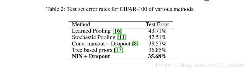
The CIFAR-100 dataset [12] is the same in size and format as the CIFAR-10 dataset, but it contains 100 classes. Thus the number of images in each class is only one tenth of the CIFAR-10 dataset. For CIFAR-100 we do not tune the hyper-parameters, but use the same setting as the CIFAR-10 dataset. The only difference is that the last mlpconv layer outputs 100 feature maps. A test error of 35.68% is obtained for CIFAR-100 which surpasses the current best performance without data augmentation by more than one percent. Details of the performance comparison are shown in Table 2.

CIFAR-100数据集[12]的大小和格式与CIFAR-10数据集相同，但它包含100个类。因此，每个类中的图像数量仅为CIFAR-10数据集的十分之一。对于CIFAR-100，我们不调优超参数，而是使用与CIFAR-10数据集相同的设置。唯一的区别是最后一个mlpconv层输出100个功能映射。CIFAR-100的测试误差为35.68%，在不增加数据的情况下，其性能优于目前的最佳性能。CIFAR-100的测试误差为35.68%，在不增加数据的情况下，其性能优于目前的最佳性能。

4.4 Street View House Numbers（街景房号）

The SVHN dataset [13] is composed of 630,420 32x32 color images, divided into training set, testing set and an extra set. The task of this data set is to classify the digit located at the center of each image. The training and testing procedure follow Goodfellow et al. [8]. Namely 400 samples per class selected from the training set and 200 samples per class from the extra set are used for validation. The remainder of the training set and the extra set are used for training. The validation

set is only used as a guidance for hyper-parameter selection, but never used for training the model.

SVHN数据集[13]由630420张32x32彩色图像组成，分为训练集、测试集和额外集。该数据集的任务是对位于每幅图像中心的数字进行分类。训练和测试程序遵循古德费罗等人的要求[8]。也就是说，从训练集中选择的每类400个样本和从额外集合中选出的每类200个样本用于验证。训练集的其余部分和额外集用于培训。验证集仅用作超参数选择的指导，而从未用于模型的训练。

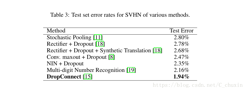
Preprocessing of the dataset again follows Goodfellow et al. [8], which was a local contrast normalization. The structure and parameters used in SVHN are similar to those used for CIFAR-10, which consist of three mlpconv layers followed by global average pooling. For this dataset, we obtain a test error rate of 2.35%. We compare our result with methods that did not augment the data, and the comparison is shown in Table 3.

数据集的预处理也同Goodfellow[8]，即使用局部对比度归一化（local contrast normalization）。Svhn中使用的结构和参数类似于CIFAR-10的结构和参数，也是由三个mlpconv层和之后的全局平均池组成。我们在这个数据集上得到2.35%的错误率。我们将结果与其他没有做数据增强的方法结果进行比较，如表3所示。

4.5 MNIST

The MNIST [1] dataset consists of hand written digits 0-9 which are 28x28 in size. There are 60,000 training images and 10,000 testing images in total. For this dataset, the same network structure as used for CIFAR-10 is adopted. But the numbers of feature maps generated from each mlpconv layer are reduced. Because MNIST is a simpler dataset compared with CIFAR-10; fewer parameters are needed. We test our method on this dataset without data augmentation. The result is compared with previous works that adopted convolutional structures, and are shown in Table 4.

MNIST[1]数据集由大小为28x28的手写数字0-9组成。共有6万张培训图像和1万张测试图像。对于这个数据集，采用了与CIFAR-10相同的网络结构.但是，从每个mlpconv层生成的特征映射的数量减少了。因为mnist是一个比CIFAR-10更简单的数据集，所以需要更少的参数。我们在这个数据集上测试我们的方法而不增加数据。计算结果与以往采用卷积结构的工作结果进行了比较，如表4所示。

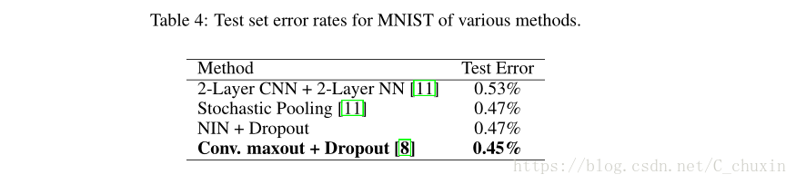
We achieve comparable but not better performance (0.47%) than the current best (0.45%) since MNIST has been tuned to a very low error rate.

我们得到了0.47%的表现，但是没有当前最好的0.45%好，因为MNIST的错误率已经非常低了。

4.6 Global Average Pooling as a Regularizer（作为正则化者的全局平均池）

Global average pooling layer is similar to the fully connected layer in that they both perform linear transformations of the vectorized feature maps. The difference lies in the transformation matrix. For global average pooling, the transformation matrix is prefixed and it is non-zero only on block diagonal elements which share the same value. Fully connected layers can have dense transformation matrices and the values are subject to back-propagation optimization. To study the regularization effect of global average pooling, we replace the global average pooling layer with a fully connected layer, while the other parts of the model remain the same. We evaluated this model with and without dropout before the fully connected linear layer. Both models are tested on the CIFAR-10 dataset,

and a comparison of the performances is shown in Table 5.

全局平均池层与完全连接层相似，因为它们都执行矢量化特征映射的线性转换。差别在于变换矩阵。对于全局平均池，变换矩阵是前缀的（ prefixed），并且仅在共享相同值的块对角线元素上是非零的。完全连通的层可以有密集的变换矩阵，并且这些值要经过反向传播优化。为了研究全局平均池的正则化效应，我们将全局平均池层替换为完全连通层，而模型的其他部分保持不变。为了研究全局平均池的正则化效应，我们将全局平均池层替换为完全连通层，而模型的其他部分保持不变。这两种模型都在CIFAR-10数据集上进行了测试，性能比较见表5。

As is shown in Table 5, the fully connected layer without dropout regularization gave the worst performance (11.59%). This is expected as the fully connected layer overfits to the training data if no regularizer is applied. Adding dropout before the fully connected layer reduced the testing error(10.88%). Global average pooling has achieved the lowest testing error (10.41%) among the three.

如表5所示，全连接层没有dropout的表现最差，11.59%，与预期一样，全连接层没有正则化器会过拟合。在完全连接层之前增加dropout，降低了测试误差(10.88%)。全局平均池的测试误差最低(10.41%)。

We then explore whether the global average pooling has the same regularization effect for conventional CNNs. We instantiate a conventional CNN as described by Hinton et al. [5], which consists of three convolutional layers and one local connection layer. The local connection layer generates 16 feature maps which are fed to a fully connected layer with dropout. To make the comparison fair, we reduce the number of feature map of the local connection layer from 16 to 10, since only one feature map is allowed for each category in the global average pooling scheme. An equivalent network with global average pooling is then created by replacing the dropout + fully connected layer with global average pooling. The performances were tested on the CIFAR-10 dataset.

接着，我们探讨全局平均池是否对常规CNN具有相同的正则化效果。我们实例化了传统的CNN，如Hinton等人所描述的[5]，由三个卷积层和一个局部连接层组成。局部连接层（local connection layer）生成16个特征映射，这些特征映射被馈送给一个完全连接的具有dropout的层。为了使比较公平，我们将本地连接层的特征映射从16减少到10，因为在全局平均池方案中，每个类别只允许一个特征映射。然后，通过用全局平均池替换掉完全连接的层，创建具有全局平均池的等效网络。在CIFAR-10数据集上进行了性能测试。

This CNN model with fully connected layer can only achieve the error rate of 17.56%. When dropout is added we achieve a similar performance (15.99%) as reported by Hinton et al. [5]. By replacing the fully connected layer with global average pooling in this model, we obtain the error rate of 16.46%, which is one percent improvement compared with the CNN without dropout. It again verifies the effectiveness of the global average pooling layer as a regularizer. Although it is

slightly worse than the dropout regularizer result, we argue that the global average pooling might be too demanding for linear convolution layers as it requires the linear filter with rectified activation to model the confidence maps of the categories.

这种全连通层CNN模型的误码率仅为17.56%。当加入Dropout时，我们实现了类似的性能(15.99%)，正如Hinton等人所报告的[5]。在该模型中，用全局平均池代替完全连通层，我们得到了16.46%的误差率，与无Dropout的CNN相比，误差提高了1%。再次验证了全局平均池层作为正则化层的有效性。虽然它略差于退出正则化结果，但我们认为对于线性卷积层来说，全局平均池可能要求过高，因为它需要经过修正激活的线性滤波器来建模类别的置信图。

4.7 Visualization of NIN（NIN可视化）

We explicitly enforce feature maps in the last mlpconv layer of NIN to be confidence maps of the categories by means of global average pooling, which is possible only with stronger local receptive field modeling, e.g. mlpconv in NIN. To understand how much this purpose is accomplished, we extract and directly visualize the feature maps from the last mlpconv layer of the trained model for CIFAR-10.

我们在nin的最后一个mlpconv层显式地执行特征映射，通过全局平均池将其作为类别的置信度映射，这只有通过更强的局部接受域建模(如nin中的mlpconv)才能实现。为了了解这一目的实现程度，我们从CIFAR-10训练模型的最后一个mlpconv层中提取并直接可视化了特征映射。

Figure 4 shows some examplar images and their corresponding feature maps for each of the ten categories selected from CIFAR-10 test set. It is expected that the largest activations are observed in the feature map corresponding to the ground truth category of the input image, which is explicitly enforced by global average pooling. Within the feature map of the ground truth category, it can be observed that the strongest activations appear roughly at the same region of the object in the original image. It is especially true for structured objects, such as the car in the second row of Figure 4. Note that the feature maps for the categories are trained with only category information. Better results are expected if bounding boxes of the objects are used for fine grained labels.

图4显示了从CIFAR-10测试集中选择的10个类别中的每个类别的一些示例图像及其相应的特征图。预期最大的激活（activations ）是在对应于输入图像的地面真相类别（ the ground truth category）的特征图中观察到的，这是通过全局平均池显式执行的。在地面真实类别的特征图中，可以观察到最强烈的激活出现在原始图像中物体的同一区域。对于结构化对象尤其如此，例如图4第二行中的CAR。请注意，类别的特征映射仅使用类别信息进行训练。如果使用对象的包围框作为细粒度标签，则期望得到更好的结果。

The visualization again demonstrates the effectiveness of NIN. It is achieved via a stronger local receptive field modeling using mlpconv layers. The global average pooling then enforces the learning of category level feature maps. Further exploration can be made towards general object detection.Detection results can be achieved based on the category level feature maps in the same flavor as in the scene labeling work of Farabet et al. [20].

可视化再次证明了nin的有效性。它是通过使用mlpconv层进行更强的局部接收场建模来实现的。然后，全局平均池强制学习类别级特征图。之后，可以对一般的目标检测做进一步的探索。检测结果可以基于与Farabet等人的场景标记工作相同的类别级特征图来实现。

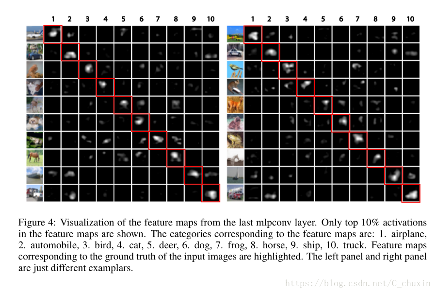
图4：最后一个mlpconv层的特征映射的可视化。只有前10%的激活功能地图显示。特征映射对应的分类如下：1.飞机，2.汽车，3.小鸟，4.猫，5.鹿，6.狗，7.青蛙，8.马，9.飞船，10.卡车。特征映射对应于输入图像的地面真相被突出显示。左面板和右面板只是不同的例子。

5 Conclusions（结论）

We proposed a novel deep network called “Network In Network” (NIN) for classification tasks. This new structure consists of mlpconv layers which use multilayer perceptrons to convolve the input and a global average pooling layer as a replacement for the fully connected layers in conventionalCNN. Mlpconv layers model the local patches better, and global average pooling acts as a structuralregularizer that prevents overfitting globally. With these two components of NIN we demonstrated state-of-the-art performance on CIFAR-10, CIFAR-100 and SVHN datasets. Through visualization of the feature maps, we demonstrated that featuremaps from the last mlpconv layer of NIN were confidence maps of the categories, and this motivates the possibility of performing object detection

via NIN.

我们提出了一种新的用于分类任务的深度网络-“网络中的网络”(NetworkinNetwork，NIN)。这种新结构由多层感知器来转换输入的mlpconv层和一个全局平均池层组成，作为传统CNN中完全连接层的替代。mlpconv层更好地模型化了局部块，全局平均池充当了防止全局过度拟合的结构正则化器。使用这两个NIN组件，我们在CIFAR-10、CIFAR-100和Svhn数据集上演示了最新的性能。通过特征映射的可视化，证明了NIN最后一个mlpconv层的特征映射是类别的置信度映射，这就激发了通过nin进行目标检测的可能性。

References（参考文献）

[1] Yann LeCun, Léon Bottou, Yoshua Bengio, and Patrick Haffner. Gradient-based learningapplied to document recognition. Proceedings of the IEEE, 86(11):2278–2324, 1998.

[2] Y Bengio, A Courville, and P Vincent. Representation learning: A review and new perspec-tives. IEEE transactions on pattern analysis and machine intelligence, 35:1798–1828, 2013.

[3] Frank Rosenblatt. Principles of neurodynamics. perceptrons and the theory of brain mechanisms. Technical report, DTIC Document, 1961.

[4] Alex Krizhevsky, Ilya Sutskever, and Geoff Hinton. Imagenet classification with deep convolutional neural networks. In Advances in Neural Information Processing Systems 25, pages 1106–1114, 2012.

[5] Geoffrey E Hinton, Nitish Srivastava, Alex Krizhevsky, Ilya Sutskever, and Ruslan R Salakhutdinov. Improving neural networks by preventing co-adaptation of feature detectors. arXiv preprint arXiv:1207.0580, 2012.

[6] Quoc V Le, Alexandre Karpenko, Jiquan Ngiam, and Andrew Ng. Ica with reconstruction cost for efficient overcomplete feature learning. In Advances in Neural Information Processing Systems, pages 1017–1025, 2011.

[7] Ian J Goodfellow. Piecewise linear multilayer perceptrons and dropout. arXiv preprint arXiv:1301.5088, 2013.

[8] Ian J Goodfellow, David Warde-Farley, Mehdi Mirza, Aaron Courville, and Yoshua Bengio. Maxout networks. arXiv preprint arXiv:1302.4389, 2013.

[9] C¸a˘ glar Gülc ¸ehre and Yoshua Bengio. Knowledge matters: Importance of prior information for optimization. arXiv preprint arXiv:1301.4083, 2013.

[10] Henry A Rowley, Shumeet Baluja, Takeo Kanade, et al. Human face detection in visual scenes. School of Computer Science, Carnegie Mellon University Pittsburgh, PA, 1995.

[11] Matthew D Zeiler and Rob Fergus. Stochastic pooling for regularization of deep convolutional neural networks. arXiv preprint arXiv:1301.3557, 2013.

[12] Alex Krizhevsky and Geoffrey Hinton. Learning multiple layers of features from tiny images.Master’s thesis, Department of Computer Science, University of Toronto, 2009.

[13] Yuval Netzer, Tao Wang, Adam Coates, Alessandro Bissacco, Bo Wu, and Andrew Y Ng. Reading digits in natural images with unsupervised feature learning. In NIPS Workshop on Deep Learning and Unsupervised Feature Learning, volume 2011, 2011.

[14] Jasper Snoek, Hugo Larochelle, and Ryan P Adams. Practical bayesian optimization of machine learning algorithms. arXiv preprint arXiv:1206.2944, 2012.

[15] Li Wan, Matthew Zeiler, Sixin Zhang, Yann L Cun, and Rob Fergus. Regularization of neural networks using dropconnect. In Proceedings of the 30th International Conference on MachineLearning (ICML-13), pages 1058–1066, 2013.

[16] Mateusz Malinowski and Mario Fritz. Learnable pooling regions for image classification. arXiv preprint arXiv:1301.3516, 2013.

[17] Nitish Srivastava and Ruslan Salakhutdinov. Discriminative transfer learning with tree-based priors. In Advances in Neural Information Processing Systems, pages 2094–2102, 2013.

[18] Nitish Srivastava. Improving neural networks with dropout. PhD thesis, University of Toronto, 2013.

[19] Ian J Goodfellow, Yaroslav Bulatov, Julian Ibarz, Sacha Arnoud, and Vinay Shet. Multi-digit number recognition from street view imagery using deep convolutional neural networks. arXiv preprint arXiv:1312.6082, 2013.

[20] Clément Farabet, Camille Couprie, Laurent Najman, Yann Lecun, et al. Learning hierarchical features for scene labeling. IEEE Transactions on Pattern Analysis and Machine Intelligence, 35:1915–1929, 2013.