知识结构

pyplot.plot()流程
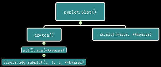
1. _axes.py中plot()函数说明
a. 调用说明
plot([x], y, [fmt], data=None, **kwargs)
plot([x], y, [fmt], [x2], y2, [fmt2], ..., **kwargs)
You can use `.Line2D` properties as keyword arguments for more
control on the  appearance. Line properties and *fmt* can be mixed.
The following two calls yield identical results:

 >>> plot(x, y, 'go--', linewidth=2, markersize=12)
 >>> plot(x, y, color='green', marker='o', linestyle='dashed',
                linewidth=2, markersize=12)
b. 参数说明
**Colors**

        The following color abbreviations are supported:

        =============    ===============================
        character        color
        =============    ===============================
        ``'b'``          blue
        ``'g'``          green
        ``'r'``          red
        ``'c'``          cyan
        ``'m'``          magenta
        ``'y'``          yellow
        ``'k'``          black
        ``'w'``          white
        =============    ===============================
**Markers**

        =============    ===============================
        character        description
        =============    ===============================
        ``'.'``          point marker
        ``','``          pixel marker
        ``'o'``          circle marker
        ``'v'``          triangle_down marker
        ``'^'``          triangle_up marker
        ``'<'``          triangle_left marker
        ``'>'``          triangle_right marker
        ``'1'``          tri_down marker
        ``'2'``          tri_up marker
        ``'3'``          tri_left marker
        ``'4'``          tri_right marker
        ``'s'``          square marker
        ``'p'``          pentagon marker
        ``'*'``          star marker
        ``'h'``          hexagon1 marker
        ``'H'``          hexagon2 marker
        ``'+'``          plus marker
        ``'x'``          x marker
        ``'D'``          diamond marker
        ``'d'``          thin_diamond marker
        ``'|'``          vline marker
        ``'_'``          hline marker
        =============    ===============================
**Line Styles**

        =============    ===============================
        character        description
        =============    ===============================
        ``'-'``          solid line style
        ``'--'``         dashed line style
        ``'-.'``         dash-dot line style
        ``':'``          dotted line style
        =============    ===============================
c. axis.plot()源码


@docstring.dedent_interpd
    def plot(self, *args, **kwargs):
        """
        Plot y versus x as lines and/or markers.

        Call signatures::

            plot([x], y, [fmt], data=None, **kwargs)
            plot([x], y, [fmt], [x2], y2, [fmt2], ..., **kwargs)

        The coordinates of the points or line nodes are given by *x*, *y*.

        The optional parameter *fmt* is a convenient way for defining basic
        formatting like color, marker and linestyle. It's a shortcut string
        notation described in the *Notes* section below.

        >>> plot(x, y)        # plot x and y using default line style and color
        >>> plot(x, y, 'bo')  # plot x and y using blue circle markers
        >>> plot(y)           # plot y using x as index array 0..N-1
        >>> plot(y, 'r+')     # ditto, but with red plusses

        You can use `.Line2D` properties as keyword arguments for more
        control on the  appearance. Line properties and *fmt* can be mixed.
        The following two calls yield identical results:

        >>> plot(x, y, 'go--', linewidth=2, markersize=12)
        >>> plot(x, y, color='green', marker='o', linestyle='dashed',
                linewidth=2, markersize=12)

        When conflicting with *fmt*, keyword arguments take precedence.

        **Plotting labelled data**

        There's a convenient way for plotting objects with labelled data (i.e.
        data that can be accessed by index ``obj['y']``). Instead of giving
        the data in *x* and *y*, you can provide the object in the *data*
        parameter and just give the labels for *x* and *y*::

        >>> plot('xlabel', 'ylabel', data=obj)

        All indexable objects are supported. This could e.g. be a `dict`, a
        `pandas.DataFame` or a structured numpy array.


        **Plotting multiple sets of data**

        There are various ways to plot multiple sets of data.

        - The most straight forward way is just to call `plot` multiple times.
          Example:

          >>> plot(x1, y1, 'bo')
          >>> plot(x2, y2, 'go')

        - Alternatively, if your data is already a 2d array, you can pass it
          directly to *x*, *y*. A separate data set will be drawn for every
          column.

          Example: an array ``a`` where the first column represents the *x*
          values and the other columns are the *y* columns::

          >>> plot(a[0], a[1:])

        - The third way is to specify multiple sets of *[x]*, *y*, *[fmt]*
          groups::

          >>> plot(x1, y1, 'g^', x2, y2, 'g-')

          In this case, any additional keyword argument applies to all
          datasets. Also this syntax cannot be combined with the *data*
          parameter.

        By default, each line is assigned a different style specified by a
        'style cycle'. The *fmt* and line property parameters are only
        necessary if you want explicit deviations from these defaults.
        Alternatively, you can also change the style cycle using the
        'axes.prop_cycle' rcParam.

        Parameters
        ----------
        x, y : array-like or scalar
            The horizontal / vertical coordinates of the data points.
            *x* values are optional. If not given, they default to
            ``[0, ..., N-1]``.

            Commonly, these parameters are arrays of length N. However,
            scalars are supported as well (equivalent to an array with
            constant value).

            The parameters can also be 2-dimensional. Then, the columns
            represent separate data sets.

        fmt : str, optional
            A format string, e.g. 'ro' for red circles. See the *Notes*
            section for a full description of the format strings.

            Format strings are just an abbreviation for quickly setting
            basic line properties. All of these and more can also be
            controlled by keyword arguments.

        data : indexable object, optional
            An object with labelled data. If given, provide the label names to
            plot in *x* and *y*.

            .. note::
                Technically there's a slight ambiguity in calls where the
                second label is a valid *fmt*. `plot('n', 'o', data=obj)`
                could be `plt(x, y)` or `plt(y, fmt)`. In such cases,
                the former interpretation is chosen, but a warning is issued.
                You may suppress the warning by adding an empty format string
                `plot('n', 'o', '', data=obj)`.


        Other Parameters
        ----------------
        scalex, scaley : bool, optional, default: True
            These parameters determined if the view limits are adapted to
            the data limits. The values are passed on to `autoscale_view`.

        **kwargs : `.Line2D` properties, optional
            *kwargs* are used to specify properties like a line label (for
            auto legends), linewidth, antialiasing, marker face color.
            Example::

            >>> plot([1,2,3], [1,2,3], 'go-', label='line 1', linewidth=2)
            >>> plot([1,2,3], [1,4,9], 'rs',  label='line 2')

            If you make multiple lines with one plot command, the kwargs
            apply to all those lines.

            Here is a list of available `.Line2D` properties:

            %(Line2D)s

        Returns
        -------
        lines
            A list of `.Line2D` objects representing the plotted data.


        See Also
        --------
        scatter : XY scatter plot with markers of variing size and/or color (
            sometimes also called bubble chart).


        Notes
        -----
        **Format Strings**

        A format string consists of a part for color, marker and line::

            fmt = '[color][marker][line]'

        Each of them is optional. If not provided, the value from the style
        cycle is used. Exception: If ``line`` is given, but no ``marker``,
        the data will be a line without markers.

        **Colors**

        The following color abbreviations are supported:

        =============    ===============================
        character        color
        =============    ===============================
        ``'b'``          blue
        ``'g'``          green
        ``'r'``          red
        ``'c'``          cyan
        ``'m'``          magenta
        ``'y'``          yellow
        ``'k'``          black
        ``'w'``          white
        =============    ===============================

        If the color is the only part of the format string, you can
        additionally use any  `matplotlib.colors` spec, e.g. full names
        (``'green'``) or hex strings (``'#008000'``).

        **Markers**

        =============    ===============================
        character        description
        =============    ===============================
        ``'.'``          point marker
        ``','``          pixel marker
        ``'o'``          circle marker
        ``'v'``          triangle_down marker
        ``'^'``          triangle_up marker
        ``'<'``          triangle_left marker
        ``'>'``          triangle_right marker
        ``'1'``          tri_down marker
        ``'2'``          tri_up marker
        ``'3'``          tri_left marker
        ``'4'``          tri_right marker
        ``'s'``          square marker
        ``'p'``          pentagon marker
        ``'*'``          star marker
        ``'h'``          hexagon1 marker
        ``'H'``          hexagon2 marker
        ``'+'``          plus marker
        ``'x'``          x marker
        ``'D'``          diamond marker
        ``'d'``          thin_diamond marker
        ``'|'``          vline marker
        ``'_'``          hline marker
        =============    ===============================

        **Line Styles**

        =============    ===============================
        character        description
        =============    ===============================
        ``'-'``          solid line style
        ``'--'``         dashed line style
        ``'-.'``         dash-dot line style
        ``':'``          dotted line style
        =============    ===============================

        Example format strings::

            'b'    # blue markers with default shape
            'ro'   # red circles
            'g-'   # green solid line
            '--'   # dashed line with default color
            'k^:'  # black triangle_up markers connected by a dotted line

        """
        scalex = kwargs.pop('scalex', True)
        scaley = kwargs.pop('scaley', True)

        if not self._hold:
            self.cla()
        lines = []

        kwargs = cbook.normalize_kwargs(kwargs, _alias_map)

        for line in self._get_lines(*args, **kwargs):
            self.add_line(line)
            lines.append(line)

        self.autoscale_view(scalex=scalex, scaley=scaley)
        return lines
pyplot.subplot()说明
subplot()函数用参数设置分区模式和当前子图,只有当前子图受到命令的影响。函数的参数有三个整数组成:第一个数字决定图形沿垂直方向被分为几部分,第二个数字决定图形沿水平方向被分为几部分,第三个数字设定可以直接用命令控制的子图
def subplot(*args, **kwargs):
    """
    Return a subplot axes at the given grid position.

    Call signature::

       subplot(nrows, ncols, index, **kwargs)

    In the current figure, create and return an `.Axes`, at position *index*
    of a (virtual) grid of *nrows* by *ncols* axes.  Indexes go from 1 to
    ``nrows * ncols``, incrementing in row-major order.

    If *nrows*, *ncols* and *index* are all less than 10, they can also be
    given as a single, concatenated, three-digit number.

    For example, ``subplot(2, 3, 3)`` and ``subplot(233)`` both create an
    `.Axes` at the top right corner of the current figure, occupying half of
    the figure height and a third of the figure width.

    .. note::

       Creating a subplot will delete any pre-existing subplot that overlaps
       with it beyond sharing a boundary::

          import matplotlib.pyplot as plt
          # plot a line, implicitly creating a subplot(111)
          plt.plot([1,2,3])
          # now create a subplot which represents the top plot of a grid
          # with 2 rows and 1 column. Since this subplot will overlap the
          # first, the plot (and its axes) previously created, will be removed
          plt.subplot(211)
          plt.plot(range(12))
          plt.subplot(212, facecolor='y') # creates 2nd subplot with yellow background

       If you do not want this behavior, use the
       :meth:`~matplotlib.figure.Figure.add_subplot` method or the
       :func:`~matplotlib.pyplot.axes` function instead.

    Keyword arguments:

      *facecolor*:
        The background color of the subplot, which can be any valid
        color specifier.  See :mod:`matplotlib.colors` for more
        information.

      *polar*:
        A boolean flag indicating whether the subplot plot should be
        a polar projection.  Defaults to *False*.

      *projection*:
        A string giving the name of a custom projection to be used
        for the subplot. This projection must have been previously
        registered. See :mod:`matplotlib.projections`.

    .. seealso::

        :func:`~matplotlib.pyplot.axes`
            For additional information on :func:`axes` and
            :func:`subplot` keyword arguments.

        :file:`gallery/pie_and_polar_charts/polar_scatter.py`
            For an example

    **Example:**

    .. plot:: gallery/subplots_axes_and_figures/subplot.py

    """
    # if subplot called without arguments, create subplot(1,1,1)
    if len(args)==0:
        args=(1,1,1)

    # This check was added because it is very easy to type
    # subplot(1, 2, False) when subplots(1, 2, False) was intended
    # (sharex=False, that is). In most cases, no error will
    # ever occur, but mysterious behavior can result because what was
    # intended to be the sharex argument is instead treated as a
    # subplot index for subplot()
    if len(args) >= 3 and isinstance(args[2], bool) :
        warnings.warn("The subplot index argument to subplot() appears"
                      " to be a boolean. Did you intend to use subplots()?")

    fig = gcf()
    a = fig.add_subplot(*args, **kwargs)
    bbox = a.bbox
    byebye = []
    for other in fig.axes:
        if other==a: continue
        if bbox.fully_overlaps(other.bbox):
            byebye.append(other)
    for ax in byebye: delaxes(ax)

    return a
figure.py/add_subplot
def add_subplot(self, *args, **kwargs):
        """
        Add a subplot.

        Parameters
        ----------
        *args
            Either a 3-digit integer or three separate integers
            describing the position of the subplot. If the three
            integers are R, C, and P in order, the subplot will take
            the Pth position on a grid with R rows and C columns.

        projection : ['aitoff' | 'hammer' | 'lambert' |
'mollweide' | 'polar' | 'rectilinear'], optional
            The projection type of the axes.

        polar : boolean, optional
            If True, equivalent to projection='polar'.

        **kwargs
            This method also takes the keyword arguments for
            :class:`~matplotlib.axes.Axes`.

        Returns
        -------
        axes : Axes
            The axes of the subplot.

        Notes
        -----
        If the figure already has a subplot with key (*args*,
        *kwargs*) then it will simply make that subplot current and
        return it.  This behavior is deprecated.

        Examples
        --------
        ::

            fig.add_subplot(111)

            # equivalent but more general
            fig.add_subplot(1, 1, 1)

            # add subplot with red background
            fig.add_subplot(212, facecolor='r')

            # add a polar subplot
            fig.add_subplot(111, projection='polar')

            # add Subplot instance sub
            fig.add_subplot(sub)

        See Also
        --------
        matplotlib.pyplot.subplot : for an explanation of the args.
        """
        if not len(args):
            return

        if len(args) == 1 and isinstance(args[0], int):
            if not 100 <= args[0] <= 999:
                raise ValueError("Integer subplot specification must be a "
                                 "three-digit number, not {}".format(args[0]))
            args = tuple(map(int, str(args[0])))

        if isinstance(args[0], SubplotBase):

            a = args[0]
            if a.get_figure() is not self:
                raise ValueError(
                    "The Subplot must have been created in the present figure")
            # make a key for the subplot (which includes the axes object id
            # in the hash)
            key = self._make_key(*args, **kwargs)
        else:
            projection_class, kwargs, key = process_projection_requirements(
                self, *args, **kwargs)

            # try to find the axes with this key in the stack
            ax = self._axstack.get(key)

            if ax is not None:
                if isinstance(ax, projection_class):
                    # the axes already existed, so set it as active & return
                    self.sca(ax)
                    return ax
                else:
                    # Undocumented convenience behavior:
                    # subplot(111); subplot(111, projection='polar')
                    # will replace the first with the second.
                    # Without this, add_subplot would be simpler and
                    # more similar to add_axes.
                    self._axstack.remove(ax)

            a = subplot_class_factory(projection_class)(self, *args, **kwargs)
        self._axstack.add(key, a)
        self.sca(a)
        a._remove_method = self.__remove_ax
        self.stale = True
        a.stale_callback = _stale_figure_callback
        return a
if subplot called without arguments, create subplot(1,1,1)
Either a 3-digit integer or three separate integers,describing the position of the subplot. If the three,integers are R, C, and P in order, the subplot will take,the Pth position on a grid with R rows and C columns.
pyplot.text()
return gca().set_title(s, *args, **kwargs)
def set_title(self, label, fontdict=None, loc="center", pad=None,
                    **kwargs):
        """
        Set a title for the axes.

        Set one of the three available axes titles. The available titles
        are positioned above the axes in the center, flush with the left
        edge, and flush with the right edge.

        Parameters
        ----------
        label : str
            Text to use for the title

        fontdict : dict
            A dictionary controlling the appearance of the title text,
            the default `fontdict` is::

               {'fontsize': rcParams['axes.titlesize'],
                'fontweight' : rcParams['axes.titleweight'],
                'verticalalignment': 'baseline',
                'horizontalalignment': loc}

        loc : {'center', 'left', 'right'}, str, optional
            Which title to set, defaults to 'center'

        pad : float
            The offset of the title from the top of the axes, in points.
            Default is ``None`` to use rcParams['axes.titlepad'].

        Returns
        -------
        text : :class:`~matplotlib.text.Text`
            The matplotlib text instance representing the title

        Other Parameters
        ----------------
        **kwargs : `~matplotlib.text.Text` properties
            Other keyword arguments are text properties, see
            :class:`~matplotlib.text.Text` for a list of valid text
            properties.
        """
        try:
            title = {'left': self._left_title,
                     'center': self.title,
                     'right': self._right_title}[loc.lower()]
        except KeyError:
            raise ValueError("'%s' is not a valid location" % loc)
        default = {
            'fontsize': rcParams['axes.titlesize'],
            'fontweight': rcParams['axes.titleweight'],
            'verticalalignment': 'baseline',
            'horizontalalignment': loc.lower()}
        if pad is None:
            pad = rcParams['axes.titlepad']
        self._set_title_offset_trans(float(pad))
        title.set_text(label)
        title.update(default)
        if fontdict is not None:
            title.update(fontdict)
        title.update(kwargs)
        return title
def text(self, x, y, s, fontdict=None, withdash=False, **kwargs)
def text(self, x, y, s, fontdict=None, withdash=False, **kwargs):
        """
        Add text to the axes.

        Add the text *s* to the axes at location *x*, *y* in data coordinates.

        Parameters
        ----------
        x, y : scalars
            The position to place the text. By default, this is in data
            coordinates. The coordinate system can be changed using the
            *transform* parameter.

        s : str
            The text.

        fontdict : dictionary, optional, default: None
            A dictionary to override the default text properties. If fontdict
            is None, the defaults are determined by your rc parameters.

        withdash : boolean, optional, default: False
            Creates a `~matplotlib.text.TextWithDash` instance instead of a
            `~matplotlib.text.Text` instance.

        Returns
        -------
        text : `.Text`
            The created `.Text` instance.

        Other Parameters
        ----------------
        **kwargs : `~matplotlib.text.Text` properties.
            Other miscellaneous text parameters.

        Examples
        --------
        Individual keyword arguments can be used to override any given
        parameter::

            >>> text(x, y, s, fontsize=12)

        The default transform specifies that text is in data coords,
        alternatively, you can specify text in axis coords (0,0 is
        lower-left and 1,1 is upper-right).  The example below places
        text in the center of the axes::

            >>> text(0.5, 0.5, 'matplotlib', horizontalalignment='center',
            ...      verticalalignment='center', transform=ax.transAxes)

        You can put a rectangular box around the text instance (e.g., to
        set a background color) by using the keyword `bbox`.  `bbox` is
        a dictionary of `~matplotlib.patches.Rectangle`
        properties.  For example::

            >>> text(x, y, s, bbox=dict(facecolor='red', alpha=0.5))
        """
        default = {
            'verticalalignment': 'baseline',
            'horizontalalignment': 'left',
            'transform': self.transData,
            'clip_on': False}

        # At some point if we feel confident that TextWithDash
        # is robust as a drop-in replacement for Text and that
        # the performance impact of the heavier-weight class
        # isn't too significant, it may make sense to eliminate
        # the withdash kwarg and simply delegate whether there's
        # a dash to TextWithDash and dashlength.
        if withdash:
            t = mtext.TextWithDash(
                x=x, y=y, text=s)
        else:
            t = mtext.Text(
                x=x, y=y, text=s)

        t.update(default)
        if fontdict is not None:
            t.update(fontdict)
        t.update(kwargs)

        t.set_clip_path(self.patch)
        self._add_text(t)
        return t
>>> text(x, y, s, fontsize=12, bbox=dict(facecolor='red', alpha=0.5))
pyplot.annotate()
该函数的实现主要基于text.py文件中的Annotation类,该函数特别适用于添加注释,需要特别关注其参数
class Annotation(Text, _AnnotationBase):
    def __str__(self):
        return "Annotation(%g,%g,%s)" % (self.xy[0],
                                         self.xy[1],
                                         repr(self._text))

    @docstring.dedent_interpd
    def __init__(self, s, xy,
                 xytext=None,
                 xycoords='data',
                 textcoords=None,
                 arrowprops=None,
                 annotation_clip=None,
                 **kwargs):
        '''
        Annotate the point ``xy`` with text ``s``.

        Additional kwargs are passed to `~matplotlib.text.Text`.

        Parameters
        ----------

        s : str
            The text of the annotation

        xy : iterable
            Length 2 sequence specifying the *(x,y)* point to annotate

        xytext : iterable, optional
            Length 2 sequence specifying the *(x,y)* to place the text
            at.  If None, defaults to ``xy``.

        xycoords : str, Artist, Transform, callable or tuple, optional

            The coordinate system that ``xy`` is given in.

            For a `str` the allowed values are:

            =================   ===============================================
            Property            Description
            =================   ===============================================
            'figure points'     points from the lower left of the figure
            'figure pixels'     pixels from the lower left of the figure
            'figure fraction'   fraction of figure from lower left
            'axes points'       points from lower left corner of axes
            'axes pixels'       pixels from lower left corner of axes
            'axes fraction'     fraction of axes from lower left
            'data'              use the coordinate system of the object being
                                annotated (default)
            'polar'             *(theta,r)* if not native 'data' coordinates
            =================   ===============================================

            If a `~matplotlib.artist.Artist` object is passed in the units are
            fraction if it's bounding box.

            If a `~matplotlib.transforms.Transform` object is passed
            in use that to transform ``xy`` to screen coordinates

            If a callable it must take a
            `~matplotlib.backend_bases.RendererBase` object as input
            and return a `~matplotlib.transforms.Transform` or
            `~matplotlib.transforms.Bbox` object

            If a `tuple` must be length 2 tuple of str, `Artist`,
            `Transform` or callable objects.  The first transform is
            used for the *x* coordinate and the second for *y*.

            See :ref:`plotting-guide-annotation` for more details.

            Defaults to ``'data'``

        textcoords : str, `Artist`, `Transform`, callable or tuple, optional
            The coordinate system that ``xytext`` is given, which
            may be different than the coordinate system used for
            ``xy``.

            All ``xycoords`` values are valid as well as the following
            strings:

            =================   =========================================
            Property            Description
            =================   =========================================
            'offset points'     offset (in points) from the *xy* value
            'offset pixels'     offset (in pixels) from the *xy* value
            =================   =========================================

            defaults to the input of ``xycoords``

        arrowprops : dict, optional
            If not None, properties used to draw a
            `~matplotlib.patches.FancyArrowPatch` arrow between ``xy`` and
            ``xytext``.

            If `arrowprops` does not contain the key ``'arrowstyle'`` the
            allowed keys are:

            ==========   ======================================================
            Key          Description
            ==========   ======================================================
            width        the width of the arrow in points
            headwidth    the width of the base of the arrow head in points
            headlength   the length of the arrow head in points
            shrink       fraction of total length to 'shrink' from both ends
            ?            any key to :class:`matplotlib.patches.FancyArrowPatch`
            ==========   ======================================================

            If the `arrowprops` contains the key ``'arrowstyle'`` the
            above keys are forbidden.  The allowed values of
            ``'arrowstyle'`` are:

            ============   =============================================
            Name           Attrs
            ============   =============================================
            ``'-'``        None
            ``'->'``       head_length=0.4,head_width=0.2
            ``'-['``       widthB=1.0,lengthB=0.2,angleB=None
            ``'|-|'``      widthA=1.0,widthB=1.0
            ``'-|>'``      head_length=0.4,head_width=0.2
            ``'<-'``       head_length=0.4,head_width=0.2
            ``'<->'``      head_length=0.4,head_width=0.2
            ``'<|-'``      head_length=0.4,head_width=0.2
            ``'<|-|>'``    head_length=0.4,head_width=0.2
            ``'fancy'``    head_length=0.4,head_width=0.4,tail_width=0.4
            ``'simple'``   head_length=0.5,head_width=0.5,tail_width=0.2
            ``'wedge'``    tail_width=0.3,shrink_factor=0.5
            ============   =============================================

            Valid keys for `~matplotlib.patches.FancyArrowPatch` are:

            ===============  ==================================================
            Key              Description
            ===============  ==================================================
            arrowstyle       the arrow style
            connectionstyle  the connection style
            relpos           default is (0.5, 0.5)
            patchA           default is bounding box of the text
            patchB           default is None
            shrinkA          default is 2 points
            shrinkB          default is 2 points
            mutation_scale   default is text size (in points)
            mutation_aspect  default is 1.
            ?                any key for :class:`matplotlib.patches.PathPatch`
            ===============  ==================================================

            Defaults to None

        annotation_clip : bool, optional
            Controls the visibility of the annotation when it goes
            outside the axes area.

            If `True`, the annotation will only be drawn when the
            ``xy`` is inside the axes. If `False`, the annotation will
            always be drawn regardless of its position.

            The default is `None`, which behave as `True` only if
            *xycoords* is "data".

        Returns
        -------
        Annotation

        '''
事例
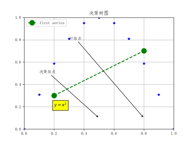
#coding=utf-8

import matplotlib.pyplot as plt
import time
import math
import numpy as np

from pylab import mpl

mpl.rcParams['font.sans-serif'] = ['FangSong'] # 指定默认字体
mpl.rcParams['axes.unicode_minus'] = False # 解决保存图像是负号'-'显示为方块的问题

def createplot():
    plt.axis([0,1,0,1])
    plt.title("决策树图")
    #plt.plot([0.2,0.8],[0.3,0.7],color='green', marker='o', linestyle='dashed',
    #            linewidth=2, markersize=12)
    plt.plot([0.2,0.8],[0.3,0.7], 'go--', linewidth=2, markersize=12)

    t = np.arange(0,2.5,0.1)
    print (t)
    y1 = list(map(math.sin, math.pi*t))
    print (y1)
    plt.plot(t, y1, 'b*')
    plt.text(0.2,0.2,r'$y=x^2$',fontsize=10, bbox={'facecolor':'yellow'})
    plt.grid(True)
    plt.legend(["first series", ],loc=2)
    #fig = plt.figure()
    #createplot.plotaxis = plt.subplot()
    plotnode(str("决策结点"),(0.5,0.1),(0.1,0.5))
    plotnode(str("叶结点"),(0.8,0.1),(0.3,0.8))
    plt.show()

def plotnode(nodetext,centerpt, textpt):
    plt.annotate(nodetext,centerpt,xytext = textpt,
    xycoords='data',arrowprops={"arrowstyle":'->'})


if __name__ == "__main__":
    createplot()
    #plotnode()