1、构建决策树的过程:
from math import log

#海洋生物数据,x1为不浮出水面是否可以生存,x2为是否有脚蹼,y为是否属于鱼类
def createDataSet():
    dataSet = [[1, 1, 'yes'],
               [1, 1, 'yes'],
               [1, 0, 'no'],
               [0, 1, 'no'],
               [0, 1, 'no']]
    labels = ['no surfacing','flippers']
    return dataSet, labels

#计算给定数据集的熵
def calcShannonEnt(dataSet):
    #计算数据集中实例的总数
    numEntries = len(dataSet)
    labelCounts = {}
    for featVec in dataSet:
        #将y取出
        currentLabel = featVec[-1]
        #创建一个数据字典,它的键值是最后一列的数值,如果当前键值不存在,则将当前键值加入字典
        if currentLabel not in labelCounts.keys(): labelCounts[currentLabel] = 0
        #每个键值都记录了当前类别出现的次数
        labelCounts[currentLabel] += 1
    shannonEnt = 0.0
    for key in labelCounts:
        #计算所有类标签发生的概率,本例:yes:2/5,no:3/5
        prob = float(labelCounts[key])/numEntries
        #计算信息熵
        shannonEnt -= prob * log(prob,2) #log base 2
    return shannonEnt

#调用
#调用函数createDataSet()
myDat,labels = createDataSet()
print('构建的数组:',myDat)
print('x的名称分别为:',labels)
#调用函数calcShannonEnt(dataSet)
p = calcShannonEnt(myDat)
print('构建的数组中y的熵:',p)
#p为熵,y中混合的数据种类越多,熵越大,下面测试这一论断
myDat[0][-1] = 'maybe'
print('对y增加一个种类,修改第一个y:',myDat)
p = calcShannonEnt(myDat)
print('对y增加一个种类,发现y的熵变大了:',p)
#恢复原样
myDat[0][-1] = 'yes'
print('将数组恢复原样:',myDat)
print('………………')

#划分数据集,使用了三个参数:待划分的数据集,划分数据集的特征,需要返回的特征的值
def splitDataSet(dataSet, axis, value):
    #创建新的列表
    retDataSet = []
    #遍历待划分的数据集
    for featVec in dataSet:
        #如果满足待划分数据集中的某个值等于需要返回的值的条件
        if featVec[axis] == value:
            #将待划分的数据集分成两部分
            reducedFeatVec = featVec[:axis]
            reducedFeatVec.extend(featVec[axis+1:])
            retDataSet.append(reducedFeatVec)
    return retDataSet

#调用,取第0个位置等于1的元素,不包括1本身
s1 = splitDataSet(myDat, 0, 1)
print('取第0个位置等于1的元素,不包括1本身:',s1)
#调用,取第0个位置等于0的元素,不包括0本身
s2 = splitDataSet(myDat, 0, 0)
print('取第0个位置等于0的元素,不包括0本身',s2)
print('………………')

#选择最好的数据集划分方式
def chooseBestFeatureToSplit(dataSet):
    #取x的种类数(columns数量)
    numFeatures = len(dataSet[0]) - 1
    #计算整个数据集的原始熵
    baseEntropy = calcShannonEnt(dataSet)
    bestInfoGain = 0.0; bestFeature = -1
    #迭代所有x的column
    for i in range(numFeatures):
        #将当前列取出
        featList = [example[i] for example in dataSet]
        #将当前列去重
        uniqueVals = set(featList)
        newEntropy = 0.0
        #迭代去重后的当前列
        for value in uniqueVals:
            #取当前列等于value的值的元素,不包括value值本身
            subDataSet = splitDataSet(dataSet, i, value)
            #当前列等于value的值的概率
            prob = len(subDataSet)/float(len(dataSet))
            #计算所有特征值的熵之和
            newEntropy += prob * calcShannonEnt(subDataSet)
        #判断信息增益,取信息增益最大的那个索引值
        infoGain = baseEntropy - newEntropy
        if (infoGain > bestInfoGain):
            bestInfoGain = infoGain
            bestFeature = i
    return bestFeature

#调用
#返回信息增益最大的那个索引值
best_x_index = chooseBestFeatureToSplit(myDat)
print('信息增益最大的那个索引值为:',best_x_index)
print('………………')

#返回出现次数最多的分类名称
import operator
def majorityCnt(classList):
    classCount={}
    for vote in classList:
        if vote not in classCount.keys(): classCount[vote] = 0
        #每个键值都记录了当前类别出现的次数
        classCount[vote] += 1
    #表示为对classCount中第1维的元素进行降序排序
    sortedClassCount = sorted(classCount.iteritems(), key=operator.itemgetter(1), reverse=True)
    return sortedClassCount[0][0]

#创建树,两个输入参数:数据集合标签列表
def createTree(dataSet,labels):
    #取y值
    classList = [example[-1] for example in dataSet]
    #代码第一个停止条件是类标签完全相同,count()函数是统计某元素出现的次数,该例为统计y中第一个数出现的次数
    if classList.count(classList[0]) == len(classList):
        return classList[0]
    #如果只有一个y的column,则返回y中出现次数最多的类别
    if len(dataSet[0]) == 1:
        return majorityCnt(classList)
    #开始创建树
    #返回信息增益最大的那个索引值
    bestFeat = chooseBestFeatureToSplit(dataSet)
    #返回信息增益最大的列名称
    bestFeatLabel = labels[bestFeat]
    myTree = {bestFeatLabel:{}}
    del(labels[bestFeat])
    #将信息增益最大的那列放到featValues中
    featValues = [example[bestFeat] for example in dataSet]
    uniqueVals = set(featValues)
    for value in uniqueVals:
        #复制所有标签,使树不会弄乱所有标签
        subLabels = labels[:]
        #运用递归,直到类标签完全相同或只有一个y的column为止
        myTree[bestFeatLabel][value] = createTree(splitDataSet(dataSet, bestFeat, value),subLabels)
    return myTree

#调用
myTree = createTree(myDat,labels)
print('将递归过程展现出来:',myTree)
print('………………')

#使用决策树执行分类,遍历整棵树,比较testVec变量中的值与树节点的值,
#如果达到叶子节点,则返回testVec位置的分类
#三个参数:第一个决策树字典,第二个x的column标签,第三个参数测试变量
def classify(inputTree,featLabels,testVec):
    firstStr = list(inputTree.keys())[0]
    secondDict = inputTree[firstStr]
    #查找当前列表中第一个匹配firstStr变量的元素
    featIndex = featLabels.index(firstStr)
    key = testVec[featIndex]
    valueOfFeat = secondDict[key]
    if isinstance(valueOfFeat, dict):
        classLabel = classify(valueOfFeat, featLabels, testVec)
    else: classLabel = valueOfFeat
    return classLabel

#调用
tree0 = {'no surfacing': {0: 'no', 1: {'flippers': {0: 'no', 1: 'yes'}}}}
labels = ['no surfacing','flippers']
print('将测试数据导入:',tree0)
print('将测试数据导入:',labels)
print('[1,0]对应的分类标签为:',classify(tree0,labels,[1,0]))
print('[1,1]对应的分类标签为:',classify(tree0,labels,[1,1]))
print('………………')

#使用pickle模块存储决策树
def storeTree(inputTree,filename):
    import pickle
    fw = open(filename,'wb')
    pickle.dump(inputTree,fw)
    fw.close()

def grabTree(filename):
    import pickle
    fr = open(filename,'rb')
    return pickle.load(fr)

#调用
storeTree(tree0,'F://python入门//文件//classifierStorage.txt')
print('将序列化对象取出:',grabTree('F://python入门//文件//classifierStorage.txt'))
结果:
构建的数组: [[1, 1, 'yes'], [1, 1, 'yes'], [1, 0, 'no'], [0, 1, 'no'], [0, 1, 'no']]
x的名称分别为: ['no surfacing', 'flippers']
构建的数组中y的熵: 0.9709505944546686
对y增加一个种类,修改第一个y: [[1, 1, 'maybe'], [1, 1, 'yes'], [1, 0, 'no'], [0, 1, 'no'], [0, 1, 'no']]
对y增加一个种类,发现y的熵变大了: 1.3709505944546687
将数组恢复原样: [[1, 1, 'yes'], [1, 1, 'yes'], [1, 0, 'no'], [0, 1, 'no'], [0, 1, 'no']]
………………
取第0个位置等于1的元素,不包括1本身: [[1, 'yes'], [1, 'yes'], [0, 'no']]
取第0个位置等于0的元素,不包括0本身 [[1, 'no'], [1, 'no']]
………………
信息增益最大的那个索引值为: 0
………………
将递归过程展现出来: {'no surfacing': {0: 'no', 1: {'flippers': {0: 'no', 1: 'yes'}}}}
………………
将测试数据导入: {'no surfacing': {0: 'no', 1: {'flippers': {0: 'no', 1: 'yes'}}}}
将测试数据导入: ['no surfacing', 'flippers']
[1,0]对应的分类标签为: no
[1,1]对应的分类标签为: yes
………………
将序列化对象取出: {'no surfacing': {0: 'no', 1: {'flippers': {0: 'no', 1: 'yes'}}}}
2、使用mapplotlib注解绘制树形图
尝试绘制一个简单的有向图:
import matplotlib.pyplot as plt
#定义决策结点形状
decisionNode = dict(boxstyle="sawtooth", fc="0.8")
#定义叶结点形状
leafNode = dict(boxstyle="round4", fc="0.8")
#设置箭头样式
arrow_args = dict(arrowstyle="<-")

#执行绘图功能
#创建绘图函数,有四个参数:文字描述,定位点(目标点),起始点,节点类型
def plotNode(nodeTxt, centerPt, parentPt, nodeType):
    #nodeTxt:(x,y)处注释文本,xy:是要添加注释的数据点的位置
    #xytext:是注释内容的位置。textcoords='axes fraction'
    #bbox:是注释框的风格和颜色深度,fc越小,注释框的颜色越深,支持输入一个字典
    #va="center",  ha="center"表示注释的坐标以注释框的正中心为准,而不是注释框的左下角(v代表垂直方向,h代表水平方向)
    #xycoords和textcoords可以指定数据点的坐标系和注释内容的坐标系(本例为距离轴坐标左下角的数字分数),通常只需指定xycoords即可,textcoords默认和xycoords相同
    #arrowprop:这个属性主要是用来画出xytext的文本坐标点到xy注释点坐标点的箭头指向线段
    createPlot.ax1.annotate(nodeTxt, xy=parentPt,  xycoords='axes fraction',
             xytext=centerPt, textcoords='axes fraction',
             va="center", ha="center", bbox=nodeType, arrowprops=arrow_args )

#创建了一个新图形并清空绘图区,然后在绘图区上绘制两个代表不同类型的树节点
def createPlot():
    #figure 命令,能够创建一个用来显示图形输出的一个窗口对象,指定了背景色为白色
    fig = plt.figure(1, facecolor='white')
    # Clear figure清除所有轴,但是窗口打开,这样它可以被重复使用。
    fig.clf()
    #subplot()用于直接指定划分方式和位置进行绘图, plt.subplot(111)表示将整个图像窗口分为1行1列, 当前位置为1
    #叠加图层时frameon必须设置成False,不然会覆盖下面的图层
    createPlot.ax1 = plt.subplot(111, frameon=False)
    plotNode('a decision node', (0.5, 0.1), (0.1, 0.5), decisionNode)
    plotNode('a leaf node', (0.8, 0.1), (0.3, 0.8), leafNode)
    plt.show()
#调用
print('尝试绘制一个简单的图形:',createPlot())
print('………………')
结果输出:

尝试绘制一个简单的图形: None
………………
绘制一个复杂的树形图:
import matplotlib.pyplot as plt
#定义决策结点形状
decisionNode = dict(boxstyle="sawtooth", fc="0.8")
#定义叶结点形状
leafNode = dict(boxstyle="round4", fc="0.8")
#设置箭头样式
arrow_args = dict(arrowstyle="<-")

#执行绘图功能
#创建绘图函数,有四个参数:文字描述,定位点(目标点),起始点,节点类型
def plotNode(nodeTxt, centerPt, parentPt, nodeType):
    #nodeTxt:(x,y)处注释文本,xy:是要添加注释的数据点的位置
    #xytext:是注释内容的位置。textcoords='axes fraction'
    #bbox:是注释框的风格和颜色深度,fc越小,注释框的颜色越深,支持输入一个字典
    #va="center",  ha="center"表示注释的坐标以注释框的正中心为准,而不是注释框的左下角(v代表垂直方向,h代表水平方向)
    #xycoords和textcoords可以指定数据点的坐标系和注释内容的坐标系(本例为距离轴坐标左下角的数字分数),通常只需指定xycoords即可,textcoords默认和xycoords相同
    #arrowprop:这个属性主要是用来画出xytext的文本坐标点到xy注释点坐标点的箭头指向线段
    createPlot.ax1.annotate(nodeTxt, xy=parentPt,  xycoords='axes fraction',
             xytext=centerPt, textcoords='axes fraction',
             va="center", ha="center", bbox=nodeType, arrowprops=arrow_args )

#创建了一个新图形并清空绘图区,然后在绘图区上绘制两个代表不同类型的树节点
#def createPlot():
#    #figure 命令,能够创建一个用来显示图形输出的一个窗口对象,指定了背景色为白色
#    fig = plt.figure(1, facecolor='white')
    # Clear figure清除所有轴,但是窗口打开,这样它可以被重复使用。
#    fig.clf()
    #subplot()用于直接指定划分方式和位置进行绘图, plt.subplot(111)表示将整个图像窗口分为1行1列, 当前位置为1
    #叠加图层时frameon必须设置成False,不然会覆盖下面的图层
#    createPlot.ax1 = plt.subplot(111, frameon=False)
#   plotNode('a decision node', (0.5, 0.1), (0.1, 0.5), decisionNode)
#    plotNode('a leaf node', (0.8, 0.1), (0.3, 0.8), leafNode)
#    plt.show()
#调用
#print('尝试绘制一个简单的图形:',createPlot())
print('………………')

#获取叶节点的数目
def getNumLeafs(myTree):
    #将叶节点数目放到numLeafs中
    numLeafs = 0
    #取第一个key值
    firstStr = list(myTree.keys())[0]
    #取第一个value值
    secondDict = myTree[firstStr]
    #遍历key值
    for key in secondDict.keys():
        #如果value值为字典,则进行此计算
        if type(secondDict[key]).__name__=='dict':
            #进行递归运算
            numLeafs += getNumLeafs(secondDict[key])
        else:   numLeafs +=1
    return numLeafs

#获取数的层数
def getTreeDepth(myTree):
    maxDepth = 0
    firstStr = list(myTree.keys())[0]
    secondDict = myTree[firstStr]
    for key in secondDict.keys():
        if type(secondDict[key]).__name__=='dict':
            thisDepth = 1 + getTreeDepth(secondDict[key])
        else:   thisDepth = 1
        if thisDepth > maxDepth: maxDepth = thisDepth
    return maxDepth

#输出预先存储的树信息
def retrieveTree(i):
    listOfTrees =[{'no surfacing': {0: 'no', 1: {'flippers': {0: 'no', 1: 'yes'}}}},
                  {'no surfacing': {0: 'no', 1: {'flippers': {0: {'head': {0: 'no', 1: 'yes'}}, 1: 'no'}}}}
                  ]
    return listOfTrees[i]

#调用
tree0 = retrieveTree(0)
print('取出一个树样例:',tree0)
print('叶节点的数目:',getNumLeafs(tree0))
print('树的层数:',getTreeDepth(tree0))
print('………………')

#计算父节点和子节点的中间位置,有三个参数:子节点位置,父节点位置,文本标签
def plotMidText(cntrPt, parentPt, txtString):
    xMid = (parentPt[0]-cntrPt[0])/2.0 + cntrPt[0]
    yMid = (parentPt[1]-cntrPt[1])/2.0 + cntrPt[1]
    createPlot.ax1.text(xMid, yMid, txtString, va="center", ha="center", rotation=30)

#绘制树形图
def plotTree(myTree, parentPt, nodeTxt):
    #将计算的叶节点放到numLeafs中
    numLeafs = getNumLeafs(myTree)
#    depth = getTreeDepth(myTree)
    #第一个节点记为firstStr
    firstStr = list(myTree.keys())[0]
    #计算子节点的位置
    cntrPt = (plotTree.xOff + (1.0 + float(numLeafs))/2.0/plotTree.totalW, plotTree.yOff)
    #计算子节点与父节点的中间位置
    plotMidText(cntrPt, parentPt, nodeTxt)
    #执行绘图功能
    plotNode(firstStr, cntrPt, parentPt, decisionNode)
    #取第一个value值
    secondDict = myTree[firstStr]
    #调整y的位置
    plotTree.yOff = plotTree.yOff - 1.0/plotTree.totalD
    #遍历子节点
    for key in secondDict.keys():
        #如果子节点的value值是字典类型
        if type(secondDict[key]).__name__=='dict':
            #进行递归
            plotTree(secondDict[key],cntrPt,str(key))
        #如果子节点的value值不是字典类型,则执行以下操作
        else:
            #增加全局变量x的偏移
            plotTree.xOff = plotTree.xOff + 1.0/plotTree.totalW
            #执行绘图功能
            plotNode(secondDict[key], (plotTree.xOff, plotTree.yOff), cntrPt, leafNode)
            #计算子节点与父节点的中间位置
            plotMidText((plotTree.xOff, plotTree.yOff), cntrPt, str(key))
    #增加全局变量y的偏移
    plotTree.yOff = plotTree.yOff + 1.0/plotTree.totalD


#准备数据
def createPlot(inTree):
    #figure 命令,能够创建一个用来显示图形输出的一个窗口对象,指定了背景色为白色
    fig = plt.figure(1, facecolor='white')
    # Clear figure清除所有轴,但是窗口打开,这样它可以被重复使用。
    fig.clf()
    axprops = dict(xticks=[], yticks=[])
    #subplot()用于直接指定划分方式和位置进行绘图, plt.subplot(111)表示将整个图像窗口分为1行1列, 当前位置为1
    #叠加图层时frameon必须设置成False,不然会覆盖下面的图层
    createPlot.ax1 = plt.subplot(111, frameon=False, **axprops)
    #存储树的宽度
    plotTree.totalW = float(getNumLeafs(inTree))
    #存储树的深度
    plotTree.totalD = float(getTreeDepth(inTree))
    #plotTree.xOff、plotTree.yOff追踪已经绘制的节点位置以及放置下一个节点的恰当位置
    plotTree.xOff = -0.5/plotTree.totalW; plotTree.yOff = 1.0;
    #调用plotTree
    plotTree(inTree, (0.5,1.0), '')
    plt.show()

#调用
myTree = retrieveTree(0)
print(createPlot(myTree))
print('………………')
myTree['no surfacing'][2] = 'maybe'
print(myTree)
print(createPlot(myTree))
结果:
………………
取出一个树样例: {'no surfacing': {0: 'no', 1: {'flippers': {0: 'no', 1: 'yes'}}}}
叶节点的数目: 3
树的层数: 2
………………
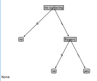
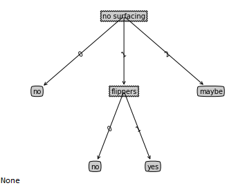
………………
{'no surfacing': {0: 'no', 1: {'flippers': {0: 'no', 1: 'yes'}}, 2: 'maybe'}}
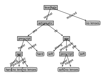
3、使用以上代码,预测隐形眼镜数据
import sys
sys.path.append(r'C://Users//91911//.spyder-py3')
import trees
#使用决策树预测隐形眼镜类型
f = open('F://python入门//文件//machinelearninginaction//Ch03//lenses.txt')
#将文本数据的每一个数据行按照tab键分割,并依次存入lenses
lenses = [inst.strip().split('	') for inst in f.readlines()]
#创建并存入特征标签列表
lensesLabels=['age','prescript','astigmatic','tearRate']
#根据继续文件得到的数据集和特征标签列表创建决策树
lensesTree=trees.createTree(lenses,lensesLabels)
print(lensesTree)from treePlotter import createPlot
#生成决策树
treePlotter.createPlot(lensesTree)
结果:
{'tearRate': {'normal': {'astigmatic': {'yes': {'prescript': {'hyper': {'age': {'young': 'hard', 'presbyopic': 'no lenses', 'pre': 'no lenses'}}, 'myope': 'hard'}}, 'no': {'age': {'young': 'soft', 'presbyopic': {'prescript': {'hyper': 'soft', 'myope': 'no lenses'}}, 'pre': 'soft'}}}}, 'reduced': 'no lenses'}}
4、一些解释说明
annotate函数详细参数解释:
    import matplotlib.pyplot as plt
    # plt.annotate(str, xy=data_point_position, xytext=annotate_position,
    #              va="center",  ha="center", xycoords="axes fraction",
    #              textcoords="axes fraction", bbox=annotate_box_type, arrowprops=arrow_style)
    # str是给数据点添加注释的内容,支持输入一个字符串
    # xy=是要添加注释的数据点的位置
    # xytext=是注释内容的位置
    # bbox=是注释框的风格和颜色深度,fc越小,注释框的颜色越深,支持输入一个字典
    # va="center",  ha="center"表示注释的坐标以注释框的正中心为准,而不是注释框的左下角(v代表垂直方向,h代表水平方向)
    # xycoords和textcoords可以指定数据点的坐标系和注释内容的坐标系,通常只需指定xycoords即可,textcoords默认和xycoords相同
    # arrowprops可以指定箭头的风格支持,输入一个字典
    # plt.annotate()的详细参数可用__doc__查看,如:print(plt.annotate.__doc__)
figure函数
matlab中的 figure 命令,能够创建一个用来显示图形输出的一个窗口对象