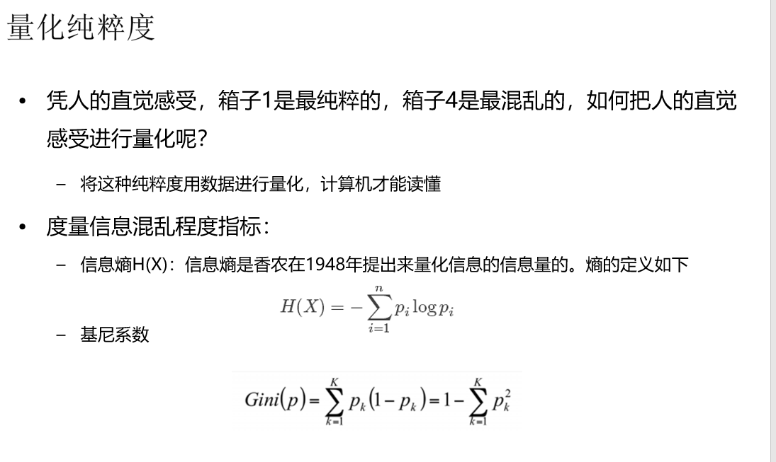
window系统
1.
anaconda  或python
spark环境变量
2.
配置spark home
D:Developspark-1.6.0-bin-hadoop2.6spark-1.6.0-bin-hadoop2.6

3.
C:UsersAdministrator>pip install py4j

python for java  cpython c 与java交互就是通过py4j

pip uninstall py4j

4.
安装pyspark (不建议pip install ,) 为了版本对应,采用复制
D:Developspark-1.6.0-bin-hadoop2.6pythonlib
py4j-0.9-src pyspark  复制到
D:DevelopPythonAnaconda3Libsite-packages

C:UsersAdministrator>python
>>> import py4j
>>> import pyspark   ## 不报错,则安装成功


idea 版本python插件下载
eclipse scala IDE 安装pydev插件

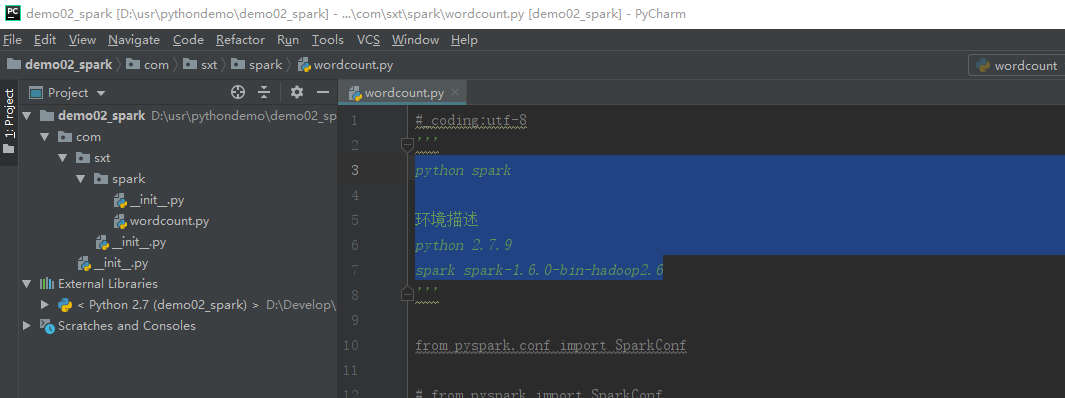
python spark

环境描述
python 2.7.9
spark spark-1.6.0-bin-hadoop2.6
安装pyspark (不建议pip install ,) 为了版本对应,采用复制,注意解压文件夹名称可能有两层,脱去外层pyspark @@@@@@@
D:Developspark-1.6.0-bin-hadoop2.6pythonlib
py4j-0.9-src pyspark  复制到
D:DevelopPythonAnaconda3Libsite-packages
安装 pyDev
pycharm  配置成功。但是不能自动提示。

scala IDE 版本太低,官网下载最新的版本,eclispe marketplace 安装老版和新版都报错。

最后:参考bing 必应搜索,【how to install pydev on eclipse scala ide】
http://www.planetofbits.com/python/how-to-install-python-pydev-plugin-in-eclipse/
重新下载 eclipse ,下载 PyDev 5.2.0 复制到eclipse dropins下。在eclispe marketplace中安装scala. ok.
eclipse 运行Python console 乱码(因为只支持gbk)


# coding:utf-8
'''
Created on 2019年10月3日

@author: Administrator

python wordcount

python print
'''
from pyspark.conf import SparkConf
from pyspark.context import SparkContext


print "hello"
print("world")

def showResult(one):
    print(one)

if __name__ == '__main__':
    conf = SparkConf()
    conf.setMaster("local")
    conf.setAppName("test")
    sc=SparkContext(conf=conf)
    lines = sc.textFile("./words")
    words = lines.flatMap(lambda line:line.split(" "))
    pairWords = words.map(lambda word:(word,1))
    reduceResult=pairWords.reduceByKey(lambda v1,v2:v1+v2)
    reduceResult.foreach(lambda one:showResult(one))
hello spark
hello hdfs
hello python
hello scala
hello hbase
hello storm
hello python
hello scala
hello hbase
hello storm
## Demo2.py
# coding:utf-8
'''
Created on 2019年10月3日

@author: Administrator
'''
from os import sys
import random
if __name__ == '__main__':
    file = sys.argv[0] ## 本文件的路径
    outputPath = sys.argv[1]
    print("%s,%s"%(file,outputPath)) ## 真正的参数

    print(random.randint(0,255)) ## 包含0和255


pvuvdata

2019-10-01	192.168.112.101	uid123214	beijing	www.taobao.com	buy
2019-10-02	192.168.112.111	uid123223	beijing	www.jingdong.com	buy
2019-10-03	192.168.112.101	uid123214	beijing	www.tencent.com	login
2019-10-04	192.168.112.101	uid123214	shanghai	www.taobao.com	buy
2019-10-01	192.168.112.101	uid123214	guangdong	www.taobao.com	logout
2019-10-01	192.168.112.101	uid123214	shanghai	www.taobao.com	view
2019-10-02	192.168.112.111	uid123223	beijing	www.jingdong.com	comment
2019-10-03	192.168.112.101	uid123214	shanghai	www.tencent.com	login
2019-10-04	192.168.112.101	uid123214	beijing	www.xiaomi.com	buy
2019-10-01	192.168.112.101	uid123214	shanghai	www.huawei.com	buy
2019-10-03	192.168.112.101	uid123214	beijing	www.tencent.com	login
2019-10-04	192.168.112.101	uid123214	shanghai	www.taobao.com	buy
2019-10-01	192.168.112.101	uid123214	guangdong	www.taobao.com	logout
2019-10-01	192.168.112.101	uid123214	beijing	www.taobao.com	view
2019-10-02	192.168.112.111	uid123223	guangdong	www.jingdong.com	comment
2019-10-03	192.168.112.101	uid123214	beijing	www.tencent.com	login
2019-10-04	192.168.112.101	uid123214	guangdong	www.xiaomi.com	buy
2019-10-01	192.168.112.101	uid123214	beijing	www.huawei.com	buy


pvuv.py
# coding:utf-8
# import sys
# print(sys.getdefaultencoding()) ## ascii
# reload(sys)
# sys.setdefaultencoding("utf-8") ## 2.x版本
# print(sys.getdefaultencoding())
from pyspark.conf import SparkConf
from pyspark.context import SparkContext
from cProfile import label
from com.sxt.spark.wordcount import showResult
'''
Created on 2019年10月3日
@author: Administrator
'''
'''
6. PySpark统计PV,UV 部分代码
1). 统计PV,UV
2). 统计除了某个地区外的UV
3).统计每个网站最活跃的top2地区
4).统计每个网站最热门的操作
5).统计每个网站下最活跃的top3用户
'''
## 方法
def pv(lines):
pairSite = lines.map(lambda line:(line.split(" ")[4],1))
reduceResult = pairSite.reduceByKey(lambda v1,v2:v1+v2)
result = reduceResult.sortBy(lambda tp:tp[1],ascending=False)
result.foreach(lambda one:showResult(one))
def uv(lines):
distinct = lines.map(lambda line:line.split(" ")[1] +'_' + line.split(" ")[4]).distinct()
reduceResult= distinct.map(lambda distinct:(distinct.split("_")[1],1)).reduceByKey(lambda v1,v2:v1+v2)
result = reduceResult.sortBy(lambda tp:tp[1],ascending=False)
result.foreach(lambda one:showResult(one))
def uvExceptBJ(lines):
distinct = lines.filter(lambda line:line.split(' ')[3]<>'beijing').map(lambda line:line.split(" ")[1] +'_' + line.split(" ")[4]).distinct()
reduceResult= distinct.map(lambda distinct:(distinct.split("_")[1],1)).reduceByKey(lambda v1,v2:v1+v2)
result = reduceResult.sortBy(lambda tp:tp[1],ascending=False)
result.foreach(lambda one:showResult(one))
def getCurrentSiteTop2Location(one):
site = one[0]
locations = one[1]
locationDict = {}
for location in locations:
if location in locationDict:
locationDict[location] +=1
else:
locationDict[location] =1
sortedList = sorted(locationDict.items(),key=lambda kv : kv[1],reverse=True)
resultList = []
if len(sortedList) < 2:
resultList = sortedList
else:
for i in range(2):
resultList.append(sortedList[i])
return site,resultList
def getTop2Location(line):
site_locations = lines.map(lambda line:(line.split(" ")[4],line.split(" ")[3])).groupByKey()
result = site_locations.map(lambda one:getCurrentSiteTop2Location(one)).collect()
for elem in result:
print(elem)
def getSiteInfo(one):
userid = one[0]
sites = one[1]
dic = {}
for site in sites:
if site in dic:
dic[site] +=1
else:
dic[site] = 1
resultList = []
for site,count in dic.items():
resultList.append((site,(userid,count)))
return resultList
'''
如下一片程序感觉有错,我写
'''
def getCurrectSiteTop3User(one):
site = one[0]
uid_c_tuples = one[1]
top3List = ["","",""]
for uid_count in uid_c_tuples:
for i in range(len(top3List)):
if top3List[i] == "":
top3List[i] = uid_count
break
else:
if uid_count[1] > top3List[i][1]: ## 元组
for j in range(2,i,-1):
top3List[j] = top3List[j-1]
top3List[i] = uid_count
break
return site,top3List
'''
如下一片程序感觉有错,老师写
'''
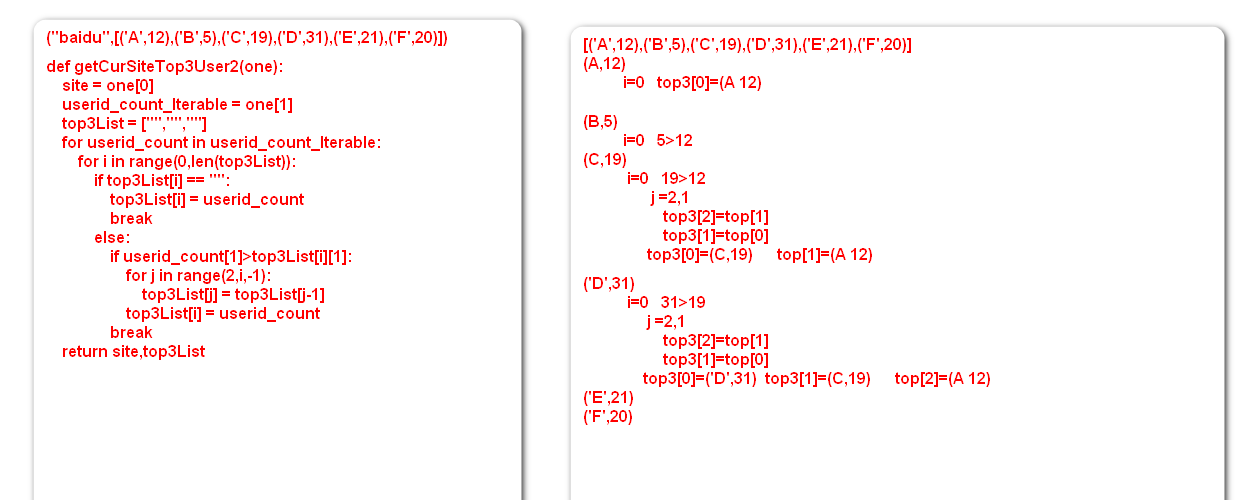
def getCurSiteTop3User2(one):
site = one[0]
userid_count_Iterable = one[1]
top3List = ["","",""]
for userid_count in userid_count_Iterable:
for i in range(0,len(top3List)):
if top3List[i] == "":
top3List[i] = userid_count
break
else:
if userid_count[1]>top3List[i][1]:
for j in range(2,i,-1):
top3List[j] = top3List[j-1]
top3List[i] = userid_count
break
return site,top3List
def getTop3User(lines):
site_uid_count = lines.map(lambda line:(line.split(' ')[2],line.split(" ")[4])).groupByKey().flatMap(lambda one:getSiteInfo(one))
result = site_uid_count.groupByKey().map(lambda one:getCurrectSiteTop3User(one)).collect()
for ele in result:
print(ele)
if __name__ == '__main__':
# conf = SparkConf().setMaster("local").setAppName("test")
# sc = SparkContext()
# lines = sc.textFile("./pvuvdata")
# # pv(lines)
# # uv(lines)
# # uvExceptBJ(lines)
# # getTop2Location(lines)
#
# getTop3User(lines)
res = getCurrectSiteTop3User(("baidu",[('A',12),('B',5),('C',12),('D',1),('E',21),('F',20)]))
print(res)
res2 = getCurSiteTop3User2(("baidu",[('A',12),('B',5),('C',12),('D',1),('E',21),('F',20)]))
print(res)
python pycharm anaconda 版本切换为3.5

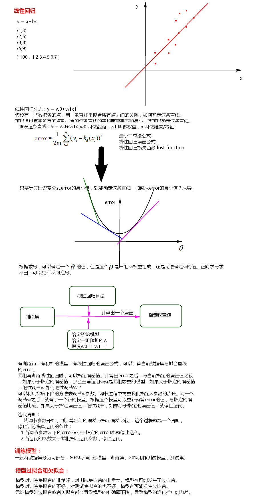
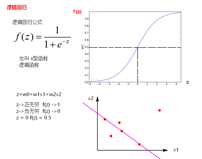
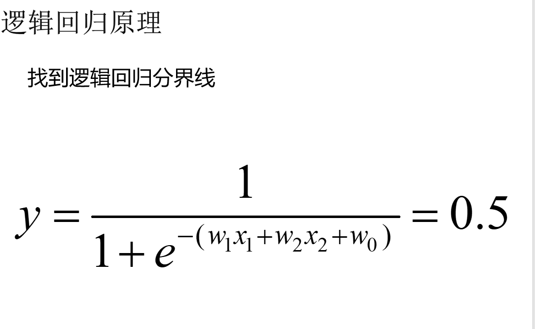
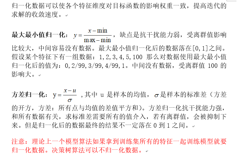
线性回归:y=w0+w1x1+w2x2...
xi称为特征,wi称为权重
矩阵转置就是矩阵旋转90度

有监督训练:是有y值;无监督训练是无y值
线性回归代码

lpsa.data

-0.4307829,-1.63735562648104 -2.00621178480549 -1.86242597251066 -1.02470580167082 -0.522940888712441 -0.863171185425945 -1.04215728919298 -0.864466507337306
-0.1625189,-1.98898046126935 -0.722008756122123 -0.787896192088153 -1.02470580167082 -0.522940888712441 -0.863171185425945 -1.04215728919298 -0.864466507337306
-0.1625189,-1.57881887548545 -2.1887840293994 1.36116336875686 -1.02470580167082 -0.522940888712441 -0.863171185425945 0.342627053981254 -0.155348103855541
-0.1625189,-2.16691708463163 -0.807993896938655 -0.787896192088153 -1.02470580167082 -0.522940888712441 -0.863171185425945 -1.04215728919298 -0.864466507337306
0.3715636,-0.507874475300631 -0.458834049396776 -0.250631301876899 -1.02470580167082 -0.522940888712441 -0.863171185425945 -1.04215728919298 -0.864466507337306
0.7654678,-2.03612849966376 -0.933954647105133 -1.86242597251066 -1.02470580167082 -0.522940888712441 -0.863171185425945 -1.04215728919298 -0.864466507337306
0.8544153,-0.557312518810673 -0.208756571683607 -0.787896192088153 0.990146852537193 -0.522940888712441 -0.863171185425945 -1.04215728919298 -0.864466507337306
1.2669476,-0.929360463147704 -0.0578991819441687 0.152317365781542 -1.02470580167082 -0.522940888712441 -0.863171185425945 -1.04215728919298 -0.864466507337306
1.2669476,-2.28833047634983 -0.0706369432557794 -0.116315079324086 0.80409888772376 -0.522940888712441 -0.863171185425945 -1.04215728919298 -0.864466507337306
1.2669476,0.223498042876113 -1.41471935455355 -0.116315079324086 -1.02470580167082 -0.522940888712441 -0.29928234305568 0.342627053981254 0.199211097885341
1.3480731,0.107785900236813 -1.47221551299731 0.420949810887169 -1.02470580167082 -0.522940888712441 -0.863171185425945 0.342627053981254 -0.687186906466865
1.446919,0.162180092313795 -1.32557369901905 0.286633588334355 -1.02470580167082 -0.522940888712441 -0.863171185425945 -1.04215728919298 -0.864466507337306
1.4701758,-1.49795329918548 -0.263601072284232 0.823898478545609 0.788388310173035 -0.522940888712441 -0.29928234305568 0.342627053981254 0.199211097885341
1.4929041,0.796247055396743 0.0476559407005752 0.286633588334355 -1.02470580167082 -0.522940888712441 0.394013435896129 -1.04215728919298 -0.864466507337306
1.5581446,-1.62233848461465 -0.843294091975396 -3.07127197548598 -1.02470580167082 -0.522940888712441 -0.863171185425945 -1.04215728919298 -0.864466507337306
1.5993876,-0.990720665490831 0.458513517212311 0.823898478545609 1.07379746308195 -0.522940888712441 -0.863171185425945 -1.04215728919298 -0.864466507337306
1.6389967,-0.171901281967138 -0.489197399065355 -0.65357996953534 -1.02470580167082 -0.522940888712441 -0.863171185425945 -1.04215728919298 -0.864466507337306
1.6956156,-1.60758252338831 -0.590700340358265 -0.65357996953534 -0.619561070667254 -0.522940888712441 -0.863171185425945 -1.04215728919298 -0.864466507337306
1.7137979,0.366273918511144 -0.414014962912583 -0.116315079324086 0.232904453212813 -0.522940888712441 0.971228997418125 0.342627053981254 1.26288870310799
1.8000583,-0.710307384579833 0.211731938156277 0.152317365781542 -1.02470580167082 -0.522940888712441 -0.442797990776478 0.342627053981254 1.61744790484887
1.8484548,-0.262791728113881 -1.16708345615721 0.420949810887169 0.0846342590816532 -0.522940888712441 0.163172393491611 0.342627053981254 1.97200710658975
1.8946169,0.899043117369237 -0.590700340358265 0.152317365781542 -1.02470580167082 -0.522940888712441 1.28643254437683 -1.04215728919298 -0.864466507337306
1.9242487,-0.903451690500615 1.07659722048274 0.152317365781542 1.28380453408541 -0.522940888712441 -0.442797990776478 -1.04215728919298 -0.864466507337306
2.008214,-0.0633337899773081 -1.38088970920094 0.958214701098423 0.80409888772376 -0.522940888712441 -0.863171185425945 -1.04215728919298 -0.864466507337306
2.0476928,-1.15393789990757 -0.961853075398404 -0.116315079324086 -1.02470580167082 -0.522940888712441 -0.442797990776478 -1.04215728919298 -0.864466507337306
2.1575593,0.0620203721138446 0.0657973885499142 1.22684714620405 -0.468824786336838 -0.522940888712441 1.31421001659859 1.72741139715549 -0.332627704725983
2.1916535,-0.75731027755674 -2.92717970468456 0.018001143228728 -1.02470580167082 -0.522940888712441 -0.863171185425945 0.342627053981254 -0.332627704725983
2.2137539,1.11226993252773 1.06484916245061 0.555266033439982 0.877691038550889 1.89254797819741 1.43890404648442 0.342627053981254 0.376490698755783
2.2772673,-0.468768642850639 -1.43754788774533 -1.05652863719378 0.576050411655607 -0.522940888712441 0.0120483832567209 0.342627053981254 -0.687186906466865
2.2975726,-0.618884859896728 -1.1366360750781 -0.519263746982526 -1.02470580167082 -0.522940888712441 -0.863171185425945 3.11219574032972 1.97200710658975
2.3272777,-0.651431999123483 0.55329161145762 -0.250631301876899 1.11210019001038 -0.522940888712441 -0.179808625688859 -1.04215728919298 -0.864466507337306
2.5217206,0.115499102435224 -0.512233676577595 0.286633588334355 1.13650173283446 -0.522940888712441 -0.179808625688859 0.342627053981254 -0.155348103855541
2.5533438,0.266341329949937 -0.551137885443386 -0.384947524429713 0.354857790686005 -0.522940888712441 -0.863171185425945 0.342627053981254 -0.332627704725983
2.5687881,1.16902610257751 0.855491905752846 2.03274448152093 1.22628985326088 1.89254797819741 2.02833774827712 3.11219574032972 2.68112551007152
2.6567569,-0.218972367124187 0.851192298581141 0.555266033439982 -1.02470580167082 -0.522940888712441 -0.863171185425945 0.342627053981254 0.908329501367106
2.677591,0.263121415733908 1.4142681068416 0.018001143228728 1.35980653053822 -0.522940888712441 -0.863171185425945 -1.04215728919298 -0.864466507337306
2.7180005,-0.0704736333296423 1.52000996595417 0.286633588334355 1.39364261119802 -0.522940888712441 -0.863171185425945 0.342627053981254 -0.332627704725983
2.7942279,-0.751957286017338 0.316843561689933 -1.99674219506348 0.911736065044475 -0.522940888712441 -0.863171185425945 -1.04215728919298 -0.864466507337306
2.8063861,-0.685277652430997 1.28214038482516 0.823898478545609 0.232904453212813 -0.522940888712441 -0.863171185425945 0.342627053981254 -0.155348103855541
2.8124102,-0.244991501432929 0.51882005949686 -0.384947524429713 0.823246560137838 -0.522940888712441 -0.863171185425945 0.342627053981254 0.553770299626224
2.8419982,-0.75731027755674 2.09041984898851 1.22684714620405 1.53428167116843 -0.522940888712441 -0.863171185425945 -1.04215728919298 -0.864466507337306
2.8535925,1.20962937075363 -0.242882661178889 1.09253092365124 -1.02470580167082 -0.522940888712441 1.24263233939889 3.11219574032972 2.50384590920108
2.9204698,0.570886990493502 0.58243883987948 0.555266033439982 1.16006887775962 -0.522940888712441 1.07357183940747 0.342627053981254 1.61744790484887
2.9626924,0.719758684343624 0.984970304132004 1.09253092365124 1.52137230773457 -0.522940888712441 -0.179808625688859 0.342627053981254 -0.509907305596424
2.9626924,-1.52406140158064 1.81975700990333 0.689582255992796 -1.02470580167082 -0.522940888712441 -0.863171185425945 -1.04215728919298 -0.864466507337306
2.9729753,-0.132431544081234 2.68769877553723 1.09253092365124 1.53428167116843 -0.522940888712441 -0.442797990776478 0.342627053981254 -0.687186906466865
3.0130809,0.436161292804989 -0.0834447307428255 -0.519263746982526 -1.02470580167082 1.89254797819741 1.07357183940747 0.342627053981254 1.26288870310799
3.0373539,-0.161195191984091 -0.671900359186746 1.7641120364153 1.13650173283446 -0.522940888712441 -0.863171185425945 0.342627053981254 0.0219314970149
3.2752562,1.39927182372944 0.513852869452676 0.689582255992796 -1.02470580167082 1.89254797819741 1.49394503405693 0.342627053981254 -0.155348103855541
3.3375474,1.51967002306341 -0.852203755696565 0.555266033439982 -0.104527297798983 1.89254797819741 1.85927724828569 0.342627053981254 0.908329501367106
3.3928291,0.560725834706224 1.87867703391426 1.09253092365124 1.39364261119802 -0.522940888712441 0.486423065822545 0.342627053981254 1.26288870310799
3.4355988,1.00765532502814 1.69426310090641 1.89842825896812 1.53428167116843 -0.522940888712441 -0.863171185425945 0.342627053981254 -0.509907305596424
3.4578927,1.10152996153577 -0.10927271844907 0.689582255992796 -1.02470580167082 1.89254797819741 1.97630171771485 0.342627053981254 1.61744790484887
3.5160131,0.100001934217311 -1.30380956369388 0.286633588334355 0.316555063757567 -0.522940888712441 0.28786643052924 0.342627053981254 0.553770299626224
3.5307626,0.987291634724086 -0.36279314978779 -0.922212414640967 0.232904453212813 -0.522940888712441 1.79270085261407 0.342627053981254 1.26288870310799
3.5652984,1.07158528137575 0.606453149641961 1.7641120364153 -0.432854616994416 1.89254797819741 0.528504607720369 0.342627053981254 0.199211097885341
3.5876769,0.180156323255198 0.188987436375017 -0.519263746982526 1.09956763075594 -0.522940888712441 0.708239632330506 0.342627053981254 0.199211097885341
3.6309855,1.65687973755377 -0.256675483533719 0.018001143228728 -1.02470580167082 1.89254797819741 1.79270085261407 0.342627053981254 1.26288870310799
3.6800909,0.5720085322365 0.239854450210939 -0.787896192088153 1.0605418233138 -0.522940888712441 -0.863171185425945 -1.04215728919298 -0.864466507337306
3.7123518,0.323806133438225 -0.606717660886078 -0.250631301876899 -1.02470580167082 1.89254797819741 0.342907418101747 0.342627053981254 0.199211097885341
3.9843437,1.23668206715898 2.54220539083611 0.152317365781542 -1.02470580167082 1.89254797819741 1.89037692416194 0.342627053981254 1.26288870310799
3.993603,0.180156323255198 0.154448192444669 1.62979581386249 0.576050411655607 1.89254797819741 0.708239632330506 0.342627053981254 1.79472750571931
4.029806,1.60906277046565 1.10378605019827 0.555266033439982 -1.02470580167082 -0.522940888712441 -0.863171185425945 -1.04215728919298 -0.864466507337306
4.1295508,1.0036214996026 0.113496885050331 -0.384947524429713 0.860016436332751 1.89254797819741 -0.863171185425945 0.342627053981254 -0.332627704725983
4.3851468,1.25591974271076 0.577607033774471 0.555266033439982 -1.02470580167082 1.89254797819741 1.07357183940747 0.342627053981254 1.26288870310799
4.6844434,2.09650591351268 0.625488598331018 -2.66832330782754 -1.02470580167082 1.89254797819741 1.67954222367555 0.342627053981254 0.553770299626224
5.477509,1.30028987435881 0.338383613253713 0.555266033439982 1.00481276295349 1.89254797819741 1.24263233939889 0.342627053981254 1.97200710658975


LinearRegression.scala

package com.bjsxt.lr

import org.apache.log4j.{ Level, Logger }
import org.apache.spark.{ SparkConf, SparkContext }
import org.apache.spark.mllib.regression.LinearRegressionWithSGD
import org.apache.spark.mllib.regression.LabeledPoint
import org.apache.spark.mllib.linalg.Vectors
import org.apache.spark.mllib.regression.LinearRegressionModel

object LinearRegression {

  def main(args: Array[String]) {
    // 构建Spark对象
    val conf = new SparkConf().setAppName("LinearRegressionWithSGD").setMaster("local")
    val sc = new SparkContext(conf)
    Logger.getRootLogger.setLevel(Level.WARN)
//        sc.setLogLevel("WARN")

    //读取样本数据
    val data_path1 = "lpsa.data"
    val data = sc.textFile(data_path1)
    val examples = data.map { line =>
      val parts = line.split(',')
      val y = parts(0)
      val xs = parts(1)
      LabeledPoint(parts(0).toDouble, Vectors.dense(parts(1).split(' ').map(_.toDouble)))
    }

    val train2TestData = examples.randomSplit(Array(0.8, 0.2), 1)

    /*
     *  迭代次数
     *  训练一个多元线性回归模型收敛(停止迭代)条件:
     *  	1、error值小于用户指定的error值
     *  	2、达到一定的迭代次数
     */
    val numIterations = 100

    //在每次迭代的过程中 梯度下降算法的下降步长大小    0.1 0.2 0.3 0.4
    val stepSize = 1


    val miniBatchFraction = 1
    val lrs = new LinearRegressionWithSGD()
    //让训练出来的模型有w0参数,就是由截距
    lrs.setIntercept(true)
    //设置步长
    lrs.optimizer.setStepSize(stepSize)
    //设置迭代次数
    lrs.optimizer.setNumIterations(numIterations)
    //每一次下山后,是否计算所有样本的误差值,1代表所有样本,默认就是1.0
    lrs.optimizer.setMiniBatchFraction(miniBatchFraction)

    val model = lrs.run(train2TestData(0))
    println(model.weights)
    println(model.intercept)

    // 对样本进行测试
    val prediction = model.predict(train2TestData(1).map(_.features))
    val predictionAndLabel = prediction.zip(train2TestData(1).map(_.label))

    val print_predict = predictionAndLabel.take(20)
    println("prediction" + "	" + "label")
    for (i <- 0 to print_predict.length - 1) {
      println(print_predict(i)._1 + "	" + print_predict(i)._2)
    }

    // 计算测试集平均误差
    val loss = predictionAndLabel.map {
      case (p, v) =>
        val err = p - v
        Math.abs(err)
    }.reduce(_ + _)
    val error = loss / train2TestData(1).count
    println("Test RMSE = " + error)
    // 模型保存
//    val ModelPath = "model"
//    model.save(sc, ModelPath)
//    val sameModel = LinearRegressionModel.load(sc, ModelPath)
    sc.stop()
  }

}

// case (p, v) 表示是 p v 结构
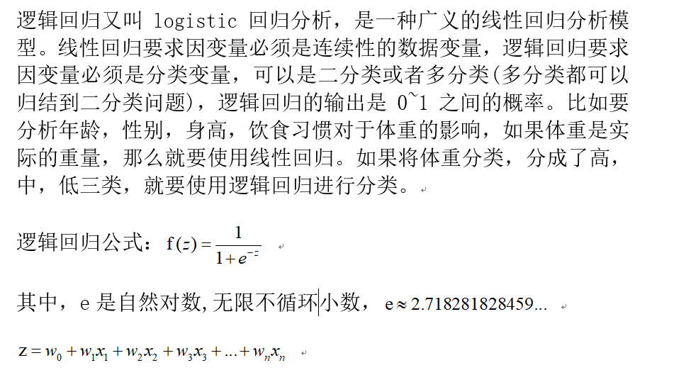
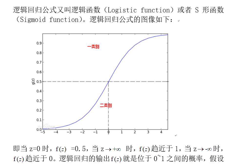
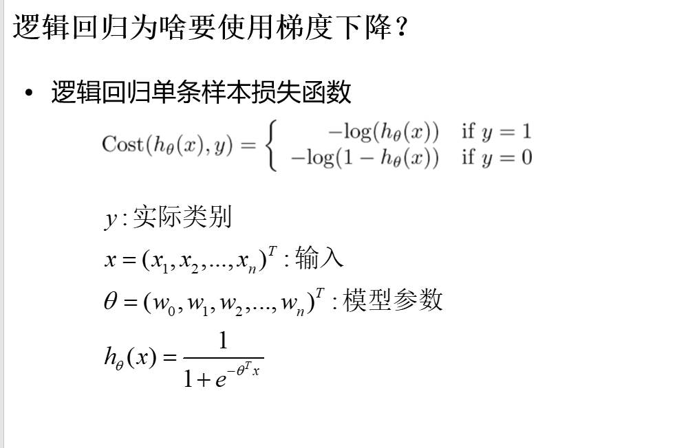
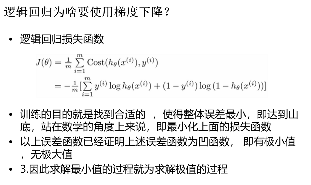
逻辑回归又称logistic回归,是一种广义的线性回归分析模型逻辑回归是一种用于分类的算法

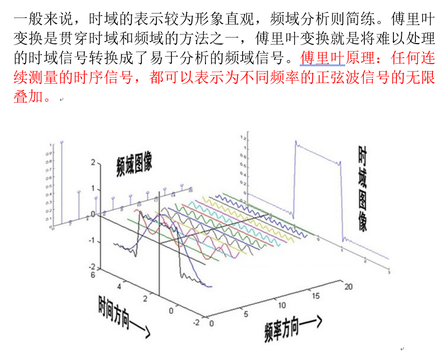
傅里叶变换:
时域分析:对一个信号来说,信号强度随时间的变化的规律就是时域特性,例如一个信号的时域波形可以表达信号随着时间的变化。
频域分析:对一个信号来说,在对其进行分析时,分析信号和频率有关的部分,而不是和时间相关的部分,和时域相对。也就是信号是由哪些单一频率的的信号合成的就是频域特性。频域中有一个重要的规则是正弦波是频域中唯一存在的波。即正弦波是对频域的描述,因为时域中的任何波形都可用正弦波合成。
一般来说,时域的表示较为形象直观,频域分析则简练。傅里叶变换是贯穿时域和频域的方法之一,傅里叶变换就是将难以处理的时域信号转换成了易于分析的频域信号。

傅里叶原理:任何连续测量的时序信号,都可以表示为不同频率的正弦波信号的无限叠加。
音乐分类的步骤:
1.	通过傅里叶变换将不同7类里面所有原始wav格式音乐文件转换为特征,并取前1000个特征,存入文件以便后续训练使用
2.	读入以上7类特征向量数据作为训练集
3.	使用sklearn包中LogisticRegression的fit方法计算出分类模型
4.	读入黑豹乐队歌曲”无地自容”并进行傅里叶变换同样取前1000维作为特征向量
5.	调用模型的predict方法对音乐进行分类,结果分为rock即摇滚类
训练集

待分类的文件

如果在python2.7下运行 需要
1,安装VCForPython27.msi
2,pip install wheel
3,pip install D:/PythonInstallPackage/numpy-1.9.2+mkl-cp27-none-win_amd64.whl
4,pip install D:/PythonInstallPackage/scipy-0.16.0-cp27-none-win_amd64.whl
5,pip install D:/PythonInstallPackage/scikit_learn-0.16.1-cp27-none-win_amd64.whl
6,pip install D:/PythonInstallPackage/python_dateutil-2.4.2-py2.py3-none-any.whl
7,pip install D:/PythonInstallPackage/six-1.9.0-py2.py3-none-any.whl
8,pip install D:/PythonInstallPackage/pyparsing-2.0.3-py2-none-any.whl
9,pip install D:/PythonInstallPackage/pytz-2015.4-py2.py3-none-any.whl
10,pip install D:/PythonInstallPackage/matplotlib-1.4.3-cp27-none-win_amd64.whl
music.py

# coding:utf-8

from scipy import fft
from scipy.io import wavfile
from matplotlib.pyplot import specgram
import matplotlib.pyplot as plt

# 可以先把一个wav文件读入python,然后绘制它的频谱图(spectrogram)来看看是什么样的

#画框设置
#figsize=(10, 4)宽度和高度的英寸
# dpi=80 分辨率
# plt.figure(figsize=(10, 4),dpi=80)
#
# (sample_rate, X) = wavfile.read("D:/usr/genres/metal/converted/metal.00065.au.wav")
# print(sample_rate, X.shape)
# specgram(X, Fs=sample_rate, xextent=(0,30))
# plt.xlabel("time")
# plt.ylabel("frequency")
# #线的形状和颜色
# plt.grid(True, linestyle='-', color='0.75')
# #tight紧凑一点
# plt.savefig("D:/usr/metal.00065.au.wav5.png", bbox_inches="tight")


# 当然,我们也可以把每一种的音乐都抽一些出来打印频谱图以便比较,如下图:
# def plotSpec(g,n):
#     sample_rate, X = wavfile.read("E:/genres/"+g+"/converted/"+g+"."+n+".au.wav")
#     specgram(X, Fs=sample_rate, xextent=(0,30))
#     plt.title(g+"_"+n[-1])
#
# plt.figure(num=None, figsize=(18, 9), dpi=80, facecolor='w', edgecolor='k')
# plt.subplot(6,3,1);plotSpec("classical","00001");plt.subplot(6,3,2);plotSpec("classical","00002")
# plt.subplot(6,3,3);plotSpec("classical","00003");plt.subplot(6,3,4);plotSpec("jazz","00001")
# plt.subplot(6,3,5);plotSpec("jazz","00002");plt.subplot(6,3,6);plotSpec("jazz","00003")
# plt.subplot(6,3,7);plotSpec("country","00001");plt.subplot(6,3,8);plotSpec("country","00002")
# plt.subplot(6,3,9);plotSpec("country","00003");plt.subplot(6,3,10);plotSpec("pop","00001")
# plt.subplot(6,3,11);plotSpec("pop","00002");plt.subplot(6,3,12);plotSpec("pop","00003")
# plt.subplot(6,3,13);plotSpec("rock","00001");plt.subplot(6,3,14);plotSpec("rock","00002")
# plt.subplot(6,3,15);plotSpec("rock","00003");plt.subplot(6,3,16);plotSpec("metal","00001")
# plt.subplot(6,3,17);plotSpec("metal","00002");plt.subplot(6,3,18);plotSpec("metal","00003")
# plt.tight_layout(pad=0.4, w_pad=0, h_pad=1.0)
# plt.savefig("D:/compare.au.wav.png", bbox_inches="tight")


# 对单首音乐进行傅里叶变换
#画框设置figsize=(9, 6)宽度和高度的英寸,dpi=80是分辨率
plt.figure(figsize=(9, 6), dpi=80)
#sample_rate代表每秒样本的采样率,X代表读取文件的所有信息 音轨信息,这里全是单音轨数据  是个数组【双音轨是个二维数组,左声道和右声道】
#采样率:每秒从连续信号中提取并组成离散信号的采样个数,它用赫兹(Hz)来表示
sample_rate, X = wavfile.read("D:/usr/genres/jazz/converted/jazz.00002.au.wav")
print(sample_rate,X,type(X),len(X))
# 大图含有2行1列共2个子图,正在绘制的是第一个
plt.subplot(211)
#画wav文件时频分析的函数
specgram(X, Fs=sample_rate)
plt.xlabel("time")
plt.ylabel("frequency")

plt.subplot(212)
#fft 快速傅里叶变换  fft(X)得到振幅 即当前采样下频率的振幅
fft_X = abs(fft(X))
print("fft_x",fft_X,len(fft_X))
#画频域分析图
specgram(fft_X)
# specgram(fft_X,Fs=1)
plt.xlabel("frequency")
plt.ylabel("amplitude")
plt.savefig("D:/usr/genres/jazz.00000.au.wav.fft.png")
plt.show()


logistic.py

# coding:utf-8

from scipy import fft
from scipy.io import wavfile
from scipy.stats import norm
from sklearn import linear_model, datasets
from sklearn.linear_model import LogisticRegression

import matplotlib.pyplot as plt
import numpy as np
"""
使用logistic regression处理音乐数据,音乐数据训练样本的获得和使用快速傅里叶变换(FFT)预处理的方法需要事先准备好
1. 把训练集扩大到每类100个首歌,类别仍然是六类:jazz,classical,country, pop, rock, metal
2. 同时使用logistic回归训练模型
3. 引入一些评价的标准来比较Logistic测试集上的表现
"""
# 准备音乐数据
def create_fft(g,n):
    rad="D:/usr/genres/"+g+"/converted/"+g+"."+str(n).zfill(5)+".au.wav"
    #sample_rate 音频的采样率,X代表读取文件的所有信息
    (sample_rate, X) = wavfile.read(rad)
    #取1000个频率特征  也就是振幅
    fft_features = abs(fft(X)[:1000])
    #zfill(5) 字符串不足5位,前面补0
    sad="D:/usr/trainset/"+g+"."+str(n).zfill(5)+ ".fft"
    np.save(sad, fft_features)

#-------create fft 构建训练集--------------

genre_list = ["classical", "jazz", "country", "pop", "rock", "metal","hiphop"]
for g in genre_list:
    for n in range(100):
        create_fft(g,n)
        print('running...')
print('finished')


#=========================================================================================
# 加载训练集数据,分割训练集以及测试集,进行分类器的训练
# 构造训练集!!!!!!!!!!!!!!!!!!!!!!!!!!!!!!!!!!!!!!!!!!!!!!!!!
#-------read fft--------------
genre_list = ["classical", "jazz", "country", "pop", "rock", "metal","hiphop"]
X=[]
Y=[]
for g in genre_list:
    for n in range(100):
        rad="D:/usr/trainset/"+g+"."+str(n).zfill(5)+ ".fft"+".npy"
        #加载文件
        fft_features = np.load(rad)
        X.append(fft_features)
        #genre_list.index(g) 返回匹配上类别的索引号
        Y.append(genre_list.index(g))

#构建的训练集
X=np.array(X)
#构建的训练集对应的类别
Y=np.array(Y)

# 接下来,我们使用sklearn,来构造和训练我们的两种分类器
#------train logistic classifier--------------
model = LogisticRegression()
#需要numpy.array类型参数
model.fit(X, Y)
print('Starting read wavfile...')
#prepare test data-------------------
# sample_rate, test = wavfile.read("i:/classical.00007.au.wav")
sample_rate, test = wavfile.read("D:/usr/projects/heibao-wudizirong-remix.wav")
print(sample_rate,test)

testdata_fft_features = abs(fft(test))[:1000]
#model.predict(testdata_fft_features) 预测为一个数组,array([类别])
print(testdata_fft_features)
# testdata_fft_features = np.array(testdata_fft_features).reshape(1, -1)
type_index = model.predict(testdata_fft_features)[0]
print(type_index)
print(genre_list[type_index])
分类结果
4
rock
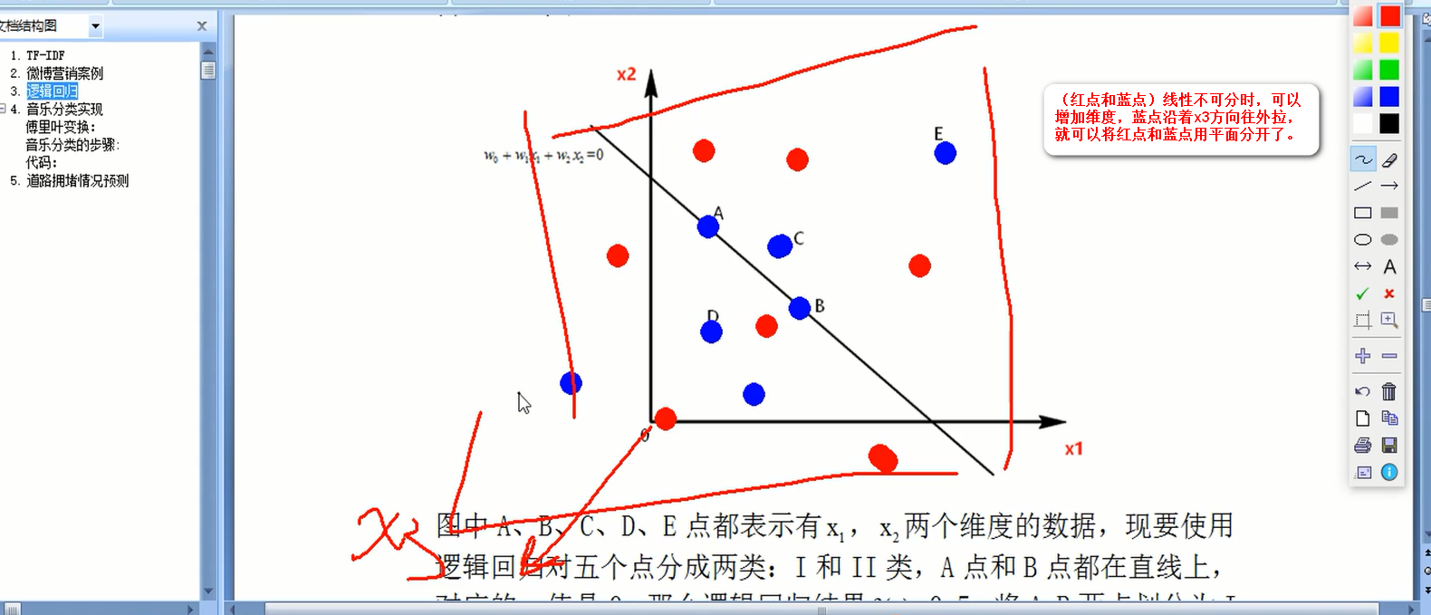
逻辑回归中:训练的模型的训练集有什么特点,训练出来的模型就有什么样的功能

思路说明
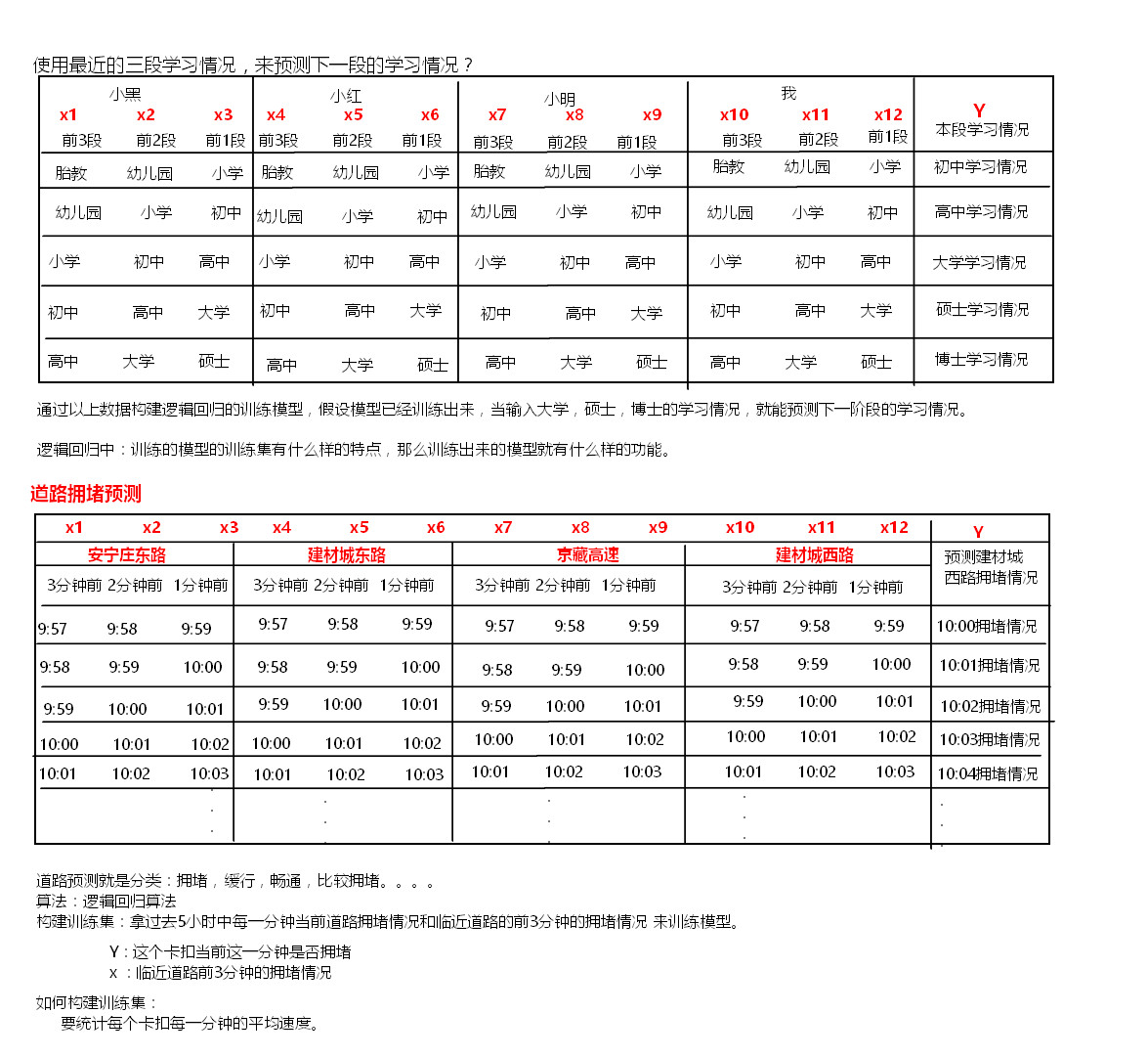
思路: 记录每一个卡口一段时间内车辆的平均速度,作为本卡口拥堵情况的分类。


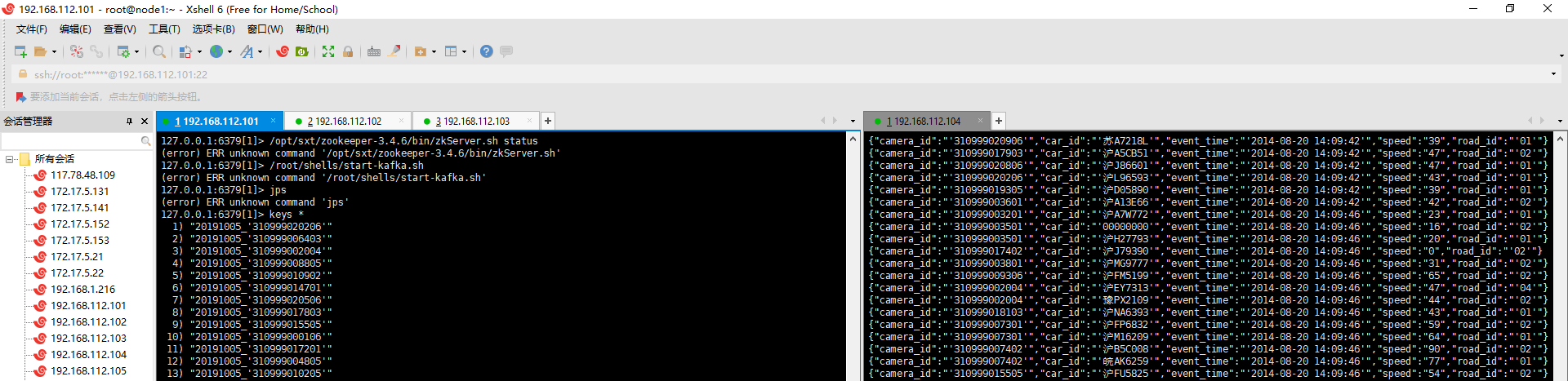
启动 zookeeper
启动 node 2,3,4 的zookeeper
/opt/sxt/zookeeper-3.4.6/bin/zkServer.sh start
启动kafka ,创建topic
node2,3,4
/root/shells/start-kafka.sh
cat start-kafka.sh
cd /opt/sxt/kafka_2.10-0.8.2.2
nohup bin/kafka-server-start.sh config/server.properties >kafka.log 2>&1 &

./bin/kafka-topics.sh -zookeeper node2:2181,node3,node4 --create --topic car_events --partitions 3 --replication-factor 3
./bin/kafka-topics.sh -zookeeper node2:2181,node3,node4 --list

./bin/kafka-console-consumer.sh --zookeeper node2,node3:2181,node4 --topic car_events

 启动  redis  redis-server  (自行百度确认)
进入redis-cli
[root@node1 ~]# redis-cli
127.0.0.1:6379> select 1
OK
127.0.0.1:6379[1]> keys *
(empty list or set)

启动spark集群
node2启动spark 集群
/opt/sxt/spark-1.6.0/sbin/start-all.sh
node3启动master集群
/opt/sxt/spark-1.6.0/sbin/start-master.sh


原始data

data/2014082013_all_column_test.txt

'310999003001', '3109990030010220140820141230292','00000000','','2014-08-20 14:09:35','0',255,'SN',  0.00,'4','','310999','310999003001','02','','','2','','','2014-08-20 14:12:30','2014-08-20 14:16:13',0,0,'2014-08-21 18:50:05','','',' '
'310999003102', '3109990031020220140820141230266','粤BT96V3','','2014-08-20 14:09:35','0',21,'NS',  0.00,'2','','310999','310999003102','02','','','2','','','2014-08-20 14:12:30','2014-08-20 14:16:13',0,0,'2014-08-21 18:50:05','','',' '
'310999000106', '3109990001060120140820141230316','沪F35253','','2014-08-20 14:09:35','0',57,'OR',  0.00,'2','','310999','310999000106','01','','','2','','','2014-08-20 14:12:30','2014-08-20 14:16:13',0,0,'2014-08-21 18:50:05','','',' '
'310999000205', '3109990002050220140820141230954','沪FN0708','','2014-08-20 14:09:35','0',33,'IR',  0.00,'2','','310999','310999000205','02','','','2','','','2014-08-20 14:12:30','2014-08-20 14:16:13',0,0,'2014-08-21 18:50:05','','',' '
'310999000205', '3109990002050120140820141230975','皖N94028','','2014-08-20 14:09:35','0',40,'IR',  0.00,'2','','310999','310999000205','01','','','2','','','2014-08-20 14:12:30','2014-08-20 14:16:13',0,0,'2014-08-21 18:50:05','','',' '
'310999015305', '3109990153050220140820141230253','沪A09L05','','2014-08-20 14:09:35','0',24,'IR',  0.00,'2','','310999','310999015305','02','','','2','','','2014-08-20 14:12:30','2014-08-20 14:16:13',0,0,'2014-08-21 18:50:05','','',' '
'310999015305', '3109990153050120140820141230658','苏FRM638','','2014-08-20 14:09:35','0',16,'IR',  0.00,'2','','310999','310999015305','01','','','2','','','2014-08-20 14:12:30','2014-08-20 14:16:13',0,0,'2014-08-21 18:50:05','','',' '
'310999003201', '3109990032010420140820141230966','沪FW3438','','2014-08-20 14:09:35','0',24,'SN',  0.00,'2','','310999','310999003201','04','','','2','','','2014-08-20 14:12:30','2014-08-20 14:16:13',0,0,'2014-08-21 18:50:05','','',' '
'310999003201', '3109990032010220140820141230302','冀F1755Z','','2014-08-20 14:09:35','0',20,'SN',  0.00,'2','','310999','310999003201','02','','','2','','','2014-08-20 14:12:30','2014-08-20 14:16:13',0,0,'2014-08-21 18:50:05','','',' '
'310999003702', '3109990037020320140820141230645','沪M05016','','2014-08-20 14:09:35','0',10,'NS',  0.00,'2','','310999','310999003702','03','','','2','','','2014-08-20 14:12:30','2014-08-20 14:16:13',0,0,'2014-08-21 18:50:05','','',' '

生产数据:
运行
package com.ic.traffic.streaming

import java.sql.Timestamp
import java.util.Properties

import kafka.javaapi.producer.Producer
import kafka.producer.{KeyedMessage, ProducerConfig}
import org.apache.spark.{SparkContext, SparkConf}
import org.codehaus.jettison.json.JSONObject

import scala.util.Random
//向kafka car_events中生产数据
object KafkaEventProducer {
  def main(args: Array[String]): Unit = {
    val topic = "car_events"
    val brokers = "node2:9092,node3:9092,node4:9092"
    val props = new Properties()
    props.put("metadata.broker.list", brokers)
    props.put("serializer.class", "kafka.serializer.StringEncoder")

    val kafkaConfig = new ProducerConfig(props)
    val producer = new Producer[String, String](kafkaConfig)

    val sparkConf = new SparkConf().setAppName("traffic data").setMaster("local[4]")
    val sc = new SparkContext(sparkConf)

    val filePath = "./data/2014082013_all_column_test.txt"

    val records = sc.textFile(filePath)
      .filter(!_.startsWith(";"))
      .map(_.split(",")).collect()

    for (i <- 1 to 100) {
      for (record <- records) {
        // prepare event data
        val event = new JSONObject()
        event.put("camera_id", record(0))
          .put("car_id", record(2))
          .put("event_time", record(4))
          .put("speed", record(6))
          .put("road_id", record(13))
        // produce event message
        producer.send(new KeyedMessage[String, String](topic,event.toString))
        println("Message sent: " + event)
        Thread.sleep(200)
      }
    }
    sc.stop
  }
}

jedis 代码
RedisClient.scala

package com.ic.traffic.streaming

import org.apache.commons.pool2.impl.GenericObjectPoolConfig
import redis.clients.jedis.JedisPool

object RedisClient extends Serializable {
  val redisHost = "node1"
  val redisPort = 6379
  val redisTimeout = 30000
  /**
   * JedisPool是一个连接池,既可以保证线程安全,又可以保证了较高的效率。
   */
  lazy val pool = new JedisPool(new GenericObjectPoolConfig(), redisHost, redisPort, redisTimeout)

//  lazy val hook = new Thread {
//    override def run = {
//      println("Execute hook thread: " + this)
//      pool.destroy()
//    }
//  }
//  sys.addShutdownHook(hook.run)
}

sparkStreaming代码
CarEventCountAnalytics.scala
package com.ic.traffic.streaming

import java.text.SimpleDateFormat
import java.util.Calendar
import kafka.serializer.StringDecoder
import net.sf.json.JSONObject
import org.apache.spark.SparkConf
import org.apache.spark.streaming._
import org.apache.spark.streaming.dstream.DStream
import org.apache.spark.streaming.kafka._
import org.apache.spark.streaming.dstream.InputDStream
/**
 * 将每个卡扣的总速度_车辆数  存入redis中
 * 【yyyyMMdd_Monitor_id,HHmm,SpeedTotal_CarCount】
 */
object CarEventCountAnalytics {

  def main(args: Array[String]): Unit = {
    // Create a StreamingContext with the given master URL
    val conf = new SparkConf().setAppName("CarEventCountAnalytics")
    if (args.length == 0) {
      conf.setMaster("local[*]")
    }
    val ssc = new StreamingContext(conf, Seconds(5))
    //    ssc.checkpoint(".")

    // Kafka configurations
    val topics = Set("car_events")
    val brokers = "node2:9092,node3:9092,node4:9092"

    val kafkaParams = Map[String, String](
      "metadata.broker.list" -> brokers,
      "serializer.class" -> "kafka.serializer.StringEncoder")


    val dbIndex = 1

    // Create a direct stream
    val kafkaStream: InputDStream[(String, String)] =
        KafkaUtils.createDirectStream[String, String, StringDecoder, StringDecoder](ssc, kafkaParams, topics)

    val events: DStream[JSONObject] = kafkaStream.map(line => {
      //JSONObject.fromObject 将string 转换成jsonObject
      val data = JSONObject.fromObject(line._2)
      println(data)
      data
    })

    /**
     * carSpeed  K:monitor_id
     * 					 V:(speedCount,carCount)
     */
    val carSpeed = events.map(jb => (jb.getString("camera_id"),jb.getInt("speed")))
                   .mapValues((speed:Int)=>(speed,1))
                   //(camera_id, (speed, 1) ) => (camera_id , (total_speed , total_count))
                   .reduceByKeyAndWindow((a:Tuple2[Int,Int], b:Tuple2[Int,Int]) => {(a._1 + b._1, a._2 + b._2)},Seconds(60),Seconds(10))
//              .reduceByKeyAndWindow((a:Tuple2[Int,Int], b:Tuple2[Int,Int]) => {(a._1 + b._1, a._2 + b._2)},(a:Tuple2[Int,Int], b:Tuple2[Int,Int]) => {(a._1 - b._1, a._2 - b._2)},Seconds(20),Seconds(10))

    carSpeed.foreachRDD(rdd => {
      rdd.foreachPartition(partitionOfRecords => {
        val jedis = RedisClient.pool.getResource
        partitionOfRecords.foreach(pair => {
          val camera_id = pair._1
          val speedTotal = pair._2._1
          val CarCount = pair._2._2
          val now = Calendar.getInstance().getTime()
          // create the date/time formatters
          val minuteFormat = new SimpleDateFormat("HHmm")
          val dayFormat = new SimpleDateFormat("yyyyMMdd")
          val time = minuteFormat.format(now)
          val day = dayFormat.format(now)
          if(CarCount!=0){
            jedis.select(dbIndex)
            jedis.hset(day + "_" + camera_id, time , speedTotal + "_" + CarCount)
          }
        })
        RedisClient.pool.returnResource(jedis)
      })
    })
    println("xxxxxxxxxxxxxxxxxxxxxxxxxxxxxxxxx")
    ssc.start()
    ssc.awaitTermination()
  }
}
接上:
启动 hdfs yarn

TrainLRwithLBFGS.scala

开始训练
package com.ic.traffic.streaming

import java.text.SimpleDateFormat
import java.util
import java.util.{Date}
import org.apache.spark.mllib.classification.LogisticRegressionWithLBFGS
import org.apache.spark.mllib.evaluation.MulticlassMetrics
import org.apache.spark.{SparkContext, SparkConf}
import org.apache.spark.mllib.linalg.Vectors
import org.apache.spark.mllib.regression.LabeledPoint
import org.apache.spark.mllib.util.MLUtils
import scala.collection.mutable.ArrayBuffer
import scala.Array
import scala.collection.mutable.ArrayBuffer
import org.apache.spark.mllib.classification.LogisticRegressionModel
/**
 * 训练模型
 */
object TrainLRwithLBFGS {

    val sparkConf = new SparkConf().setAppName("train traffic model").setMaster("local[*]")
    val sc = new SparkContext(sparkConf)

    // create the date/time formatters
    val dayFormat = new SimpleDateFormat("yyyyMMdd")
    val minuteFormat = new SimpleDateFormat("HHmm")

    def main(args: Array[String]) {

        // fetch data from redis
        val jedis = RedisClient.pool.getResource
        jedis.select(1)

        // find relative road monitors for specified road
        // val camera_ids = List("310999003001","310999003102","310999000106","310999000205","310999007204")
        val camera_ids = List("310999003001","310999003102")
        val camera_relations:Map[String,Array[String]] = Map[String,Array[String]](
            "310999003001" -> Array("310999003001","310999003102","310999000106","310999000205","310999007204"),
            "310999003102" -> Array("310999003001","310999003102","310999000106","310999000205","310999007204")
        )

        val temp = camera_ids.map({ camera_id =>
            val hours = 5
            val nowtimelong = System.currentTimeMillis();
            val now = new Date(nowtimelong)
            val day = dayFormat.format(now)//yyyyMMdd

            val array = camera_relations.get(camera_id).get

            /**
             * relations中存储了每一个卡扣在day这一天每一分钟的平均速度
             */
            val relations = array.map({ camera_id =>
//                println(camera_id)
                // fetch records of one camera for three hours ago
                val minute_speed_car_map = jedis.hgetAll(day + "_'" + camera_id+"'")
                (camera_id, minute_speed_car_map)
            })

//            relations.foreach(println)

            // organize above records per minute to train data set format (MLUtils.loadLibSVMFile)
            val dataSet = ArrayBuffer[LabeledPoint]()
            // start begin at index 3
            //Range 从300到1 递减 不包含0
            for(i <- Range(60*hours,0,-1)){
                val features = ArrayBuffer[Double]()
                val labels = ArrayBuffer[Double]()
                // get current minute and recent two minutes
                for(index <- 0 to 2){
                    //当前时刻过去的时间那一分钟
                    val tempOne = nowtimelong - 60 * 1000 * (i-index)
                    val d = new Date(tempOne)
                    val tempMinute = minuteFormat.format(d)//HHmm
                    //下一分钟
                    val tempNext = tempOne - 60 * 1000 * (-1)
                    val dNext = new Date(tempNext)
                    val tempMinuteNext = minuteFormat.format(dNext)//HHmm

                    for((k,v) <- relations){
                        val map = v //map -- k:HHmm    v:Speed
                        if(index == 2 && k == camera_id){
                            if (map.containsKey(tempMinuteNext)) {
                                val info = map.get(tempMinuteNext).split("_")
                                val f = info(0).toFloat / info(1).toFloat
                                labels += f
                            }
                        }
                        if (map.containsKey(tempMinute)){
                            val info = map.get(tempMinute).split("_")
                            val f = info(0).toFloat / info(1).toFloat
                            features += f
                        } else{
                            features += -1.0
                        }
                    }
                }

                if(labels.toArray.length == 1 ){
                    //array.head 返回数组第一个元素
                    val label = (labels.toArray).head
                    val record = LabeledPoint(if ((label.toInt/10)<10) (label.toInt/10) else 10.0, Vectors.dense(features.toArray))
                    dataSet += record
                }
            }
//            dataSet.foreach(println)
//            println(dataSet.length)

            val data = sc.parallelize(dataSet)

            // Split data into training (80%) and test (20%).
            //将data这个RDD随机分成 8:2两个RDD
            val splits = data.randomSplit(Array(0.8, 0.2))
            //构建训练集
            val training = splits(0)
            /**
             * 测试集的重要性:
             * 	测试模型的准确度,防止模型出现过拟合的问题
             */
            val test = splits(1)

            if(!data.isEmpty()){

                // 训练逻辑回归模型
                val model = new LogisticRegressionWithLBFGS()
                        .setNumClasses(11)
                        .setIntercept(true)
                        .run(training)

                // 测试集测试模型
                val predictionAndLabels = test.map { case LabeledPoint(label, features) =>
                    val prediction = model.predict(features)
                    (prediction, label)
                }

                predictionAndLabels.foreach(x=> println("预测类别:"+x._1+",真实类别:"+x._2))

                // Get evaluation metrics. 得到评价指标
                val metrics: MulticlassMetrics = new MulticlassMetrics(predictionAndLabels)
                val precision = metrics.precision// 准确率
                println("Precision = " + precision)

                if(precision > 0.8){
                    val path = "hdfs://node1:8020/model/model_"+camera_id+"_"+nowtimelong
//                    		val path = "hdfs://node1:9000/model/model_"+camera_id+"_"+nowtimelong
                    model.save(sc, path)
                    println("saved model to "+ path)
                    jedis.hset("model", camera_id , path)

                }
            }
        })
        RedisClient.pool.returnResource(jedis)
    }
}

预测 PredictLRwithLBFGS.scala    修改当前时间符合运行的时间段,在到redis 中查看效果如何。

package com.ic.traffic.streaming

import java.text.SimpleDateFormat
import java.util.Date

import org.apache.spark.mllib.classification.{ LogisticRegressionModel, LogisticRegressionWithLBFGS }
import org.apache.spark.mllib.evaluation.MulticlassMetrics
import org.apache.spark.mllib.linalg.Vectors
import org.apache.spark.mllib.regression.LabeledPoint
import org.apache.spark.{ SparkConf, SparkContext }

import scala.collection.mutable.ArrayBuffer

object PredictLRwithLBFGS {

  val sparkConf = new SparkConf().setAppName("predict traffic").setMaster("local[4]")
  val sc = new SparkContext(sparkConf)

  // create the date/time formatters
  val dayFormat = new SimpleDateFormat("yyyyMMdd")
  val minuteFormat = new SimpleDateFormat("HHmm")
  val sdf = new SimpleDateFormat("yyyy-MM-dd_HH:mm:ss")

  def main(args: Array[String]) {

    val input = "2019-10-05_01:35:00"
    val date = sdf.parse(input)
    val inputTimeLong = date.getTime()
//    val inputTime = new Date(inputTimeLong)
    val day = dayFormat.format(date)//yyyyMMdd

    // fetch data from redis
    val jedis = RedisClient.pool.getResource
    jedis.select(1)

    // find relative road monitors for specified road
    // val camera_ids = List("310999003001","310999003102","310999000106","310999000205","310999007204")
    val camera_ids = List("310999003001", "310999003102")
    val camera_relations: Map[String, Array[String]] = Map[String, Array[String]](
      "310999003001" -> Array("310999003001", "310999003102", "310999000106", "310999000205", "310999007204"),
      "310999003102" -> Array("310999003001", "310999003102", "310999000106", "310999000205", "310999007204"))

    val temp = camera_ids.map({ camera_id =>
      val list = camera_relations.get(camera_id).get

      val relations = list.map({ camera_id =>
        // fetch records of one camera for three hours ago
        (camera_id, jedis.hgetAll(day + "_'" + camera_id + "'"))
      })

//      relations.foreach(println)

      // organize above records per minute to train data set format (MLUtils.loadLibSVMFile)
      val aaa = ArrayBuffer[Double]()
      // get current minute and recent two minutes
      for (index <- 3 to (1,-1)) {
        //拿到过去 一分钟,两分钟,过去三分钟的时间戳
        val tempOne = inputTimeLong - 60 * 1000 * index
        val currentOneTime = new Date(tempOne)
        //获取输入时间的 "HHmm"
        val tempMinute = minuteFormat.format(currentOneTime)
        println("inputtime ====="+currentOneTime)
        for ((k, v) <- relations) {
          // k->camera_id ; v->speed
          val map = v
          if (map.containsKey(tempMinute)) {
            val info = map.get(tempMinute).split("_")
            val f = info(0).toFloat / info(1).toFloat
            aaa += f
          } else {
            aaa += -1.0
          }
        }
      }

      // Run training algorithm to build the model
      val path = jedis.hget("model", camera_id)
      if(path!=null){
    	    val model = LogisticRegressionModel.load(sc, path)
  			  // Compute raw scores on the test set.
  			  val prediction = model.predict(Vectors.dense(aaa.toArray))
  			  println(input + "	" + camera_id + "	" + prediction + "	")
  			  //            jedis.hset(input, camera_id, prediction.toString)
      }
    })

    RedisClient.pool.returnResource(jedis)
  }
}
127.0.0.1:6379[1]> hgetall "20191005_'310999019905'"
  1) "0103"
  2) "38_1"
  3) "0104"
  4) "179_5"
  5) "0105"
  6) "39_1"
  7) "0107"
  8) "178_5"
  9) "0108"
 10) "39_1"
逻辑回归深入以及优化
分别对应如上的 1,2,3 4 5
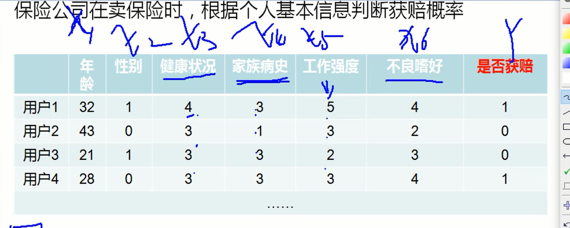
健康状况训练集.txt
1 1:57 2:0 3:0 4:5 5:3 6:5
1 1:56 2:1 3:0 4:3 5:4 6:3
1 1:27 2:0 3:0 4:4 5:3 6:4
1 1:46 2:0 3:0 4:3 5:2 6:4
1 1:75 2:1 3:0 4:3 5:3 6:2
1 1:19 2:1 3:0 4:4 5:4 6:4
1 1:49 2:0 3:0 4:4 5:3 6:3
1 1:25 2:1 3:0 4:3 5:5 6:4
1 1:47 2:1 3:0 4:3 5:4 6:3
1 1:59 2:0 3:1 4:0 5:1 6:2
1 1:18 2:0 3:0 4:4 5:3 6:3
1 1:79 2:0 3:0 4:5 5:4 6:3
LogisticRegression1.scala
package com.bjsxt.lr
import org.apache.spark.mllib.classification.{LogisticRegressionWithLBFGS}
import org.apache.spark.mllib.util.MLUtils
import org.apache.spark.{SparkConf, SparkContext}
/**
* 逻辑回归 健康状况训练集
*/
object LogisticRegression {
def main(args: Array[String]) {
val conf = new SparkConf().setAppName("spark").setMaster("local[3]")
val sc = new SparkContext(conf)
//加载 LIBSVM 格式的数据 这种格式特征前缀要从1开始
val inputData = MLUtils.loadLibSVMFile(sc, "健康状况训练集.txt")
val splits = inputData.randomSplit(Array(0.7, 0.3), seed = 1L)
val (trainingData, testData) = (splits(0), splits(1))
val lr = new LogisticRegressionWithLBFGS()
// lr.setIntercept(true)
val model = lr.run(trainingData)
val result = testData
.map{point=>Math.abs(point.label-model.predict(point.features)) }
println("正确率="+(1.0-result.mean()))
/**
*逻辑回归算法训练出来的模型,模型中的参数个数(w0....w6)=训练集中特征数(6)+1
*/
println(model.weights.toArray.mkString(" "))
println(model.intercept)
sc.stop()
}
}
w0测试数据.txt
0 1:1.0140641394573489 2:1.0053491794300906
1 1:2.012709390641638 2:2.001907117215239
0 1:1.0052568352996578 2:1.0162894218780352
1 1:2.0140249849545118 2:2.0042119386532122
0 1:1.0159829400919032 2:1.0194470820311243
1 1:2.007369501382139 2:2.0071524676923533
0 1:1.0013307693392184 2:1.0158450335581597
1 1:2.01517182545874 2:2.0052873772719177
0 1:1.0130231961501968 2:1.019126883631059
1 1:2.014080456651037 2:2.004348828637212
0 1:1.0094645373208078 2:1.0092571241891017
LogisticRegression2.scala
package com.bjsxt.lr
import org.apache.spark.mllib.classification.{LogisticRegressionWithLBFGS, LogisticRegressionWithSGD}
import org.apache.spark.mllib.regression.LabeledPoint
import org.apache.spark.mllib.util.MLUtils
import org.apache.spark.rdd.RDD
import org.apache.spark.{SparkConf, SparkContext}
/**
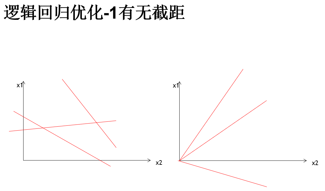
* 有无截距
*/
object LogisticRegression2 {
def main(args: Array[String]) {
val conf = new SparkConf().setAppName("spark").setMaster("local[3]")
val sc = new SparkContext(conf)
val inputData: RDD[LabeledPoint] = MLUtils.loadLibSVMFile(sc, "w0测试数据.txt")
/**
* randomSplit(Array(0.7, 0.3))方法就是将一个RDD拆分成N个RDD,N = Array.length
* 第一个RDD中的数据量和数组中的第一个元素值相关
*/
val splits = inputData.randomSplit(Array(0.7, 0.3),11L)
val (trainingData, testData) = (splits(0), splits(1))
val lr = new LogisticRegressionWithSGD
// 设置要有W0,也就是有截距
lr.setIntercept(true)
val model=lr.run(trainingData)
val result=testData.map{labeledpoint=>Math.abs(labeledpoint.label-model.predict(labeledpoint.features)) }
println("正确率="+(1.0-result.mean()))
println(model.weights.toArray.mkString(" "))
println(model.intercept)
}
}
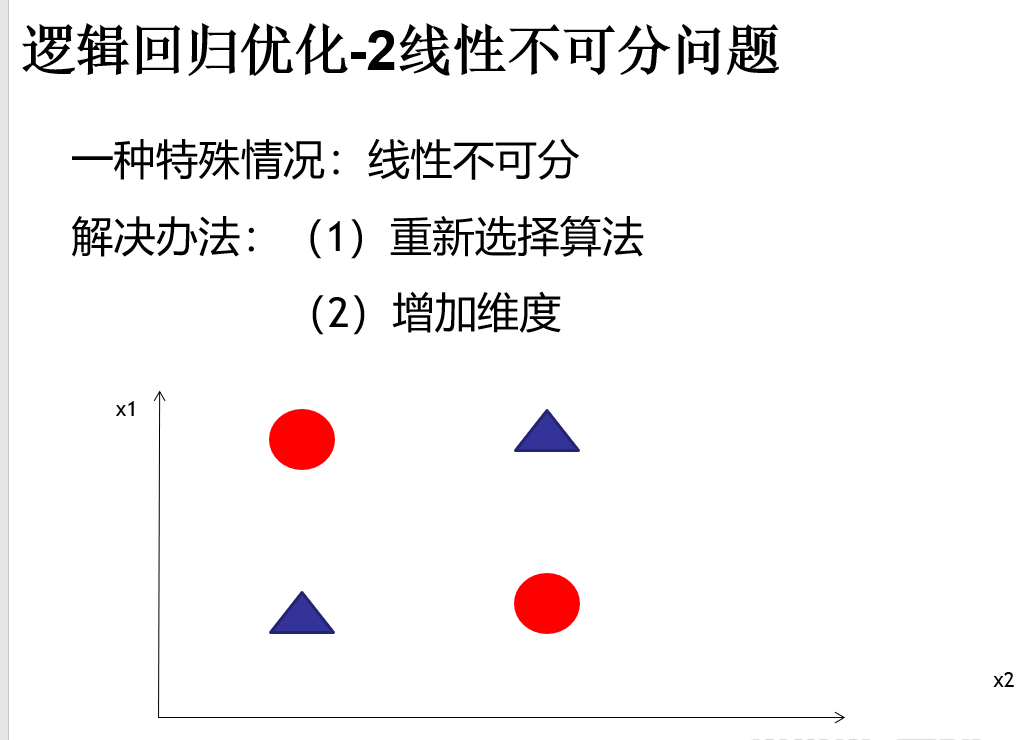
线性不可分数据集.txt
0 1:1.0021476396439248 2:1.0005277544365077
0 1:0.004780438916016197 2:0.004464089083318912
1 1:1.005957371386034 2:0.009488506452877079
1 1:0.0032888762213735202 2:1.0096142970365218
0 1:1.004487425006835 2:1.0108859204789946
0 1:0.016129088455466407 2:0.013415124039032063
1 1:1.0183108247074553 2:0.014888578069677983
1 1:0.005267064113457103 2:1.0149789230465331
0 1:1.0079616977465946 2:1.0135833360338558
0 1:0.011391932589615935 2:0.015552261205467644
LogisticRegression3.scala
package com.bjsxt.lr
import org.apache.spark.mllib.classification.{LogisticRegressionWithLBFGS, LogisticRegressionWithSGD}
import org.apache.spark.mllib.linalg.Vectors
import org.apache.spark.mllib.regression.LabeledPoint
import org.apache.spark.mllib.util.MLUtils
import org.apache.spark.{SparkConf, SparkContext}
/**
* 线性不可分 ----升高维度
*/
object LogisticRegression3 {
def main(args: Array[String]) {
val conf = new SparkConf().setAppName("spark").setMaster("local[3]")
val sc = new SparkContext(conf)
// 解决线性不可分我们来升维,升维有代价,计算复杂度变大了
val inputData = MLUtils.loadLibSVMFile(sc, "线性不可分数据集.txt")
.map { labelpoint =>
val label = labelpoint.label
val feature = labelpoint.features
//新维度的值,必须基于已有的维度值的基础上,经过一系列的数学变换得来
val array = Array(feature(0), feature(1), feature(0) * feature(1))
val convertFeature = Vectors.dense(array)
new LabeledPoint(label, convertFeature)
}
val splits = inputData.randomSplit(Array(0.7, 0.3),11L)
val (trainingData, testData) = (splits(0), splits(1))
val lr = new LogisticRegressionWithLBFGS()
lr.setIntercept(true)
val model = lr.run(trainingData)
val result = testData
.map { point => Math.abs(point.label - model.predict(point.features)) }
println("正确率=" + (1.0 - result.mean()))
println(model.weights.toArray.mkString(" "))
println(model.intercept)
}
}
健康状况训练集.txt
1 1:57 2:0 3:0 4:5 5:3 6:5
1 1:56 2:1 3:0 4:3 5:4 6:3
1 1:27 2:0 3:0 4:4 5:3 6:4
1 1:46 2:0 3:0 4:3 5:2 6:4
1 1:75 2:1 3:0 4:3 5:3 6:2
1 1:19 2:1 3:0 4:4 5:4 6:4
1 1:49 2:0 3:0 4:4 5:3 6:3
1 1:25 2:1 3:0 4:3 5:5 6:4
1 1:47 2:1 3:0 4:3 5:4 6:3
1 1:59 2:0 3:1 4:0 5:1 6:2
LogisticRegression4.scala
package com.bjsxt.lr
import org.apache.spark.mllib.classification.{LogisticRegressionWithLBFGS, LogisticRegressionWithSGD}
import org.apache.spark.mllib.util.MLUtils
import org.apache.spark.{SparkConf, SparkContext}
/**
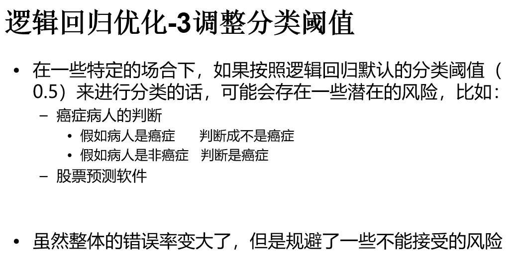
* 设置分类阈值
*/
object LogisticRegression4 {
def main(args: Array[String]) {
val conf = new SparkConf().setAppName("spark").setMaster("local[3]")
val sc = new SparkContext(conf)
/**
* LabeledPoint = Vector+Y
*/
val inputData = MLUtils.loadLibSVMFile(sc, "健康状况训练集.txt")
val splits = inputData.randomSplit(Array(0.7, 0.3),11L)
val (trainingData, testData) = (splits(0), splits(1))
val lr = new LogisticRegressionWithLBFGS()
lr.setIntercept(true)
// val model = lr.run(trainingData)
// val result = testData
// .map{point=>Math.abs(point.label-model.predict(point.features)) }
// println("正确率="+(1.0-result.mean()))
// println(model.weights.toArray.mkString(" "))
// println(model.intercept)
/**
* 如果在训练模型的时候没有调用clearThreshold这个方法,那么这个模型预测出来的结果都是分类号
* 如果在训练模型的时候调用clearThreshold这个方法,那么这个模型预测出来的结果是一个概率
*/
val model = lr.run(trainingData).clearThreshold()
val errorRate = testData.map{p=>
//score就是一个概率值
val score = model.predict(p.features)
// 癌症病人宁愿判断出得癌症也别错过一个得癌症的病人
val result = score>0.3 match {case true => 1 ; case false => 0}
Math.abs(result-p.label)
}.mean()
println(1-errorRate)
}
}
LogisticRegression5.scala
package com.bjsxt.lr
import org.apache.spark.mllib.classification.{LogisticRegressionWithLBFGS, LogisticRegressionWithSGD}
import org.apache.spark.mllib.optimization.{L1Updater, SquaredL2Updater}
import org.apache.spark.mllib.util.MLUtils
import org.apache.spark.{SparkConf, SparkContext}
/**
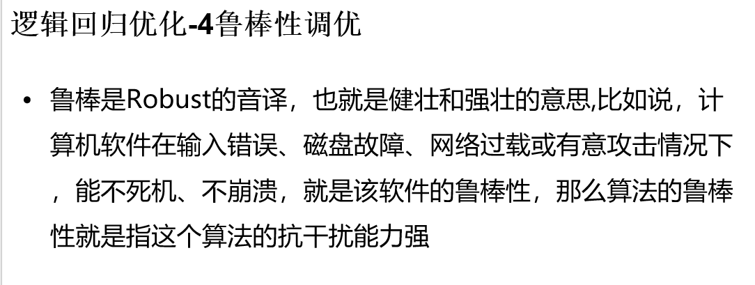
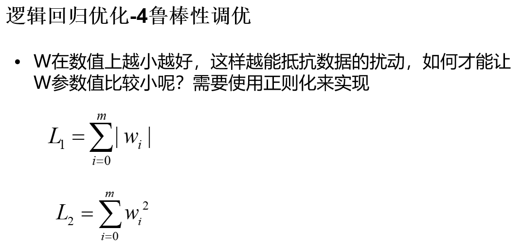
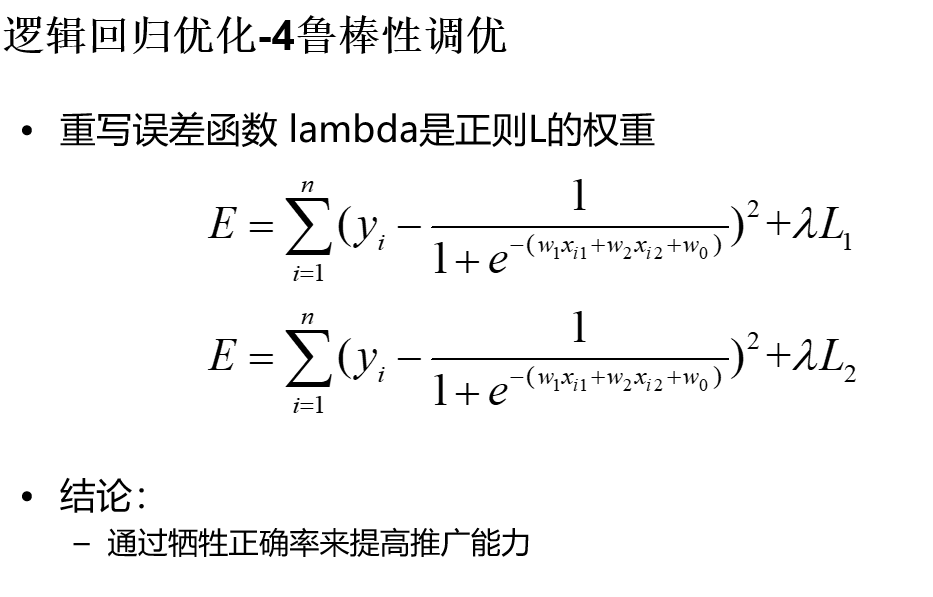
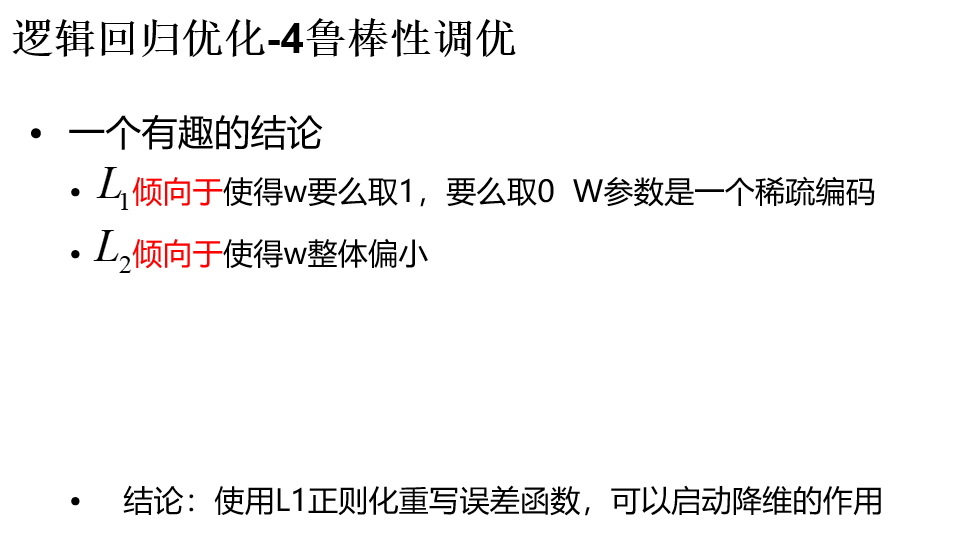
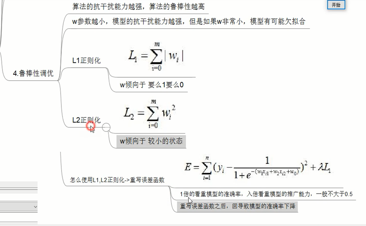
* 鲁棒性调优
* 提高模型抗干扰能力
*/
object LogisticRegression5 {
def main(args: Array[String]) {
val conf = new SparkConf().setAppName("spark").setMaster("local[3]")
val sc = new SparkContext(conf)
val inputData = MLUtils.loadLibSVMFile(sc, "健康状况训练集.txt")
val splits = inputData.randomSplit(Array(0.7, 0.3),100)
val (trainingData, testData) = (splits(0), splits(1))
/**
* LogisticRegressionWithSGD 既有L1 又有L2正则化(默认)
*/
val lr = new LogisticRegressionWithSGD()
lr.setIntercept(true)
// lr.optimizer.setUpdater(new L1Updater())
lr.optimizer.setUpdater(new SquaredL2Updater)
/**
* LogisticRegressionWithLBFGS 既有L1 又有L2正则化(默认)
*/
// val lr = new LogisticRegressionWithLBFGS()
// lr.setIntercept(true)
// lr.optimizer.setUpdater(new L1Updater)
// lr.optimizer.setUpdater(new SquaredL2Updater)
/**
* 这块设置的是我们的lambda,越大越看重这个模型的推广能力,一般不会超过1,0.4是个比较好的值
*/
lr.optimizer.setRegParam(0.4)
val model = lr.run(trainingData)
val result=testData
.map{point=>Math.abs(point.label-model.predict(point.features)) }
println("正确率="+(1.0-result.mean()))
println(model.weights.toArray.mkString(" "))
println(model.intercept)
}
}
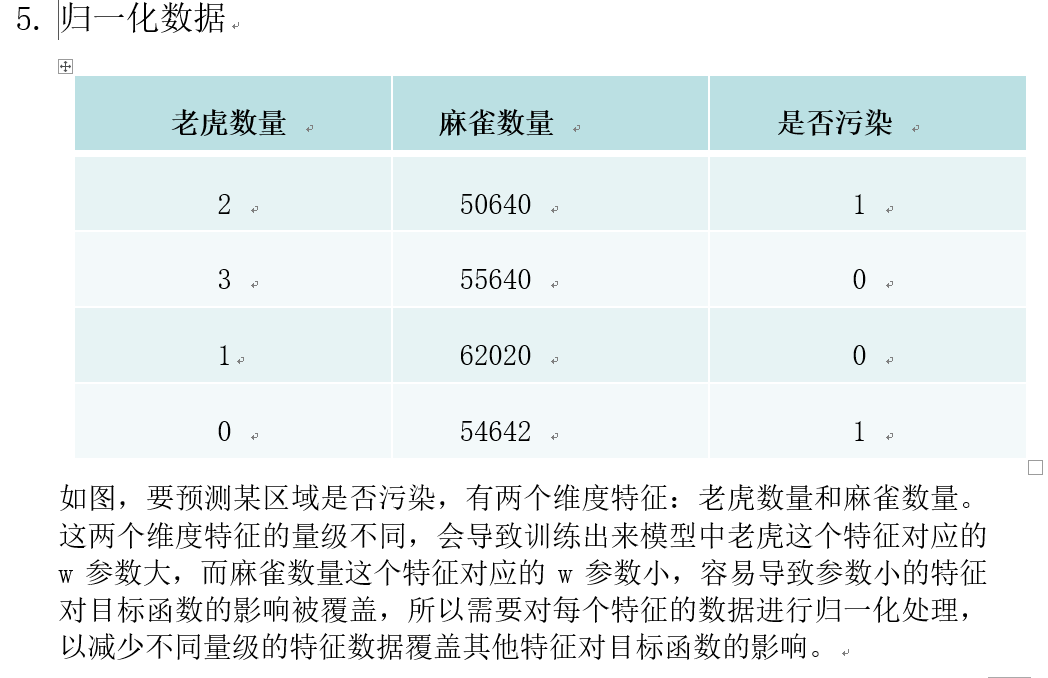
环境分类数据.txt

0 1:49 2:52320
1 1:17 2:17868
0 1:36 2:54418
1 1:13 2:19701
0 1:30 2:97516
1 1:15 2:17075
0 1:37 2:77589
1 1:10 2:14078
0 1:53 2:65912
1 1:17 2:16562
0 1:50 2:76091


LogisticRegression6.scala

package com.bjsxt.lr

import org.apache.spark.mllib.classification.{LogisticRegressionWithLBFGS, LogisticRegressionWithSGD}
import org.apache.spark.mllib.feature.StandardScaler
import org.apache.spark.mllib.regression.LabeledPoint
import org.apache.spark.mllib.util.MLUtils
import org.apache.spark.{SparkConf, SparkContext}
import org.apache.spark.ml.feature.MinMaxScaler
import org.apache.spark.sql.SQLContext
/**
 * 方差归一化
 */
object LogisticRegression6 {

  def main(args: Array[String]) {
    val conf = new SparkConf().setAppName("spark").setMaster("local[3]")
    val sc = new SparkContext(conf)
    val sqlContext = new SQLContext(sc)
    /**
     * scalerModel 这个对象中已经有每一列的均值和方差
     * withStd:代表的是方差归一化
     * withMean:代表的是均值归一化
     * scalerModel:存放每一列的方差值
     *
     * withMean默认为false, withStd默认为true
     * 当withMean=true,withStd=false时,向量中的各元素均减去它相应的均值。
     * 当withMean=true,withStd=true时,各元素在减去相应的均值之后,还要除以它们相应的标准差。
     *
     */
    val inputData = MLUtils.loadLibSVMFile(sc, "环境分类数据.txt")

    val vectors = inputData.map(_.features)
    val scalerModel = new StandardScaler(withMean=true, withStd=true).fit(vectors)

    val normalizeInputData = inputData.map{point =>
      val label = point.label
      //对每一条数据进行了归一化
      val features = scalerModel.transform(point.features.toDense)
      println(features)
      new LabeledPoint(label,features)
    }


    val splits = normalizeInputData.randomSplit(Array(0.7, 0.3),100)
    val (trainingData, testData) = (splits(0), splits(1))
    val lr=new LogisticRegressionWithLBFGS()
//    val lr = new LogisticRegressionWithSGD()
    lr.setIntercept(true)
    val model = lr.run(trainingData)
    val result=testData.map{point=>Math.abs(point.label-model.predict(point.features)) }
    println("正确率="+(1.0-result.mean()))
    println(model.weights.toArray.mkString(" "))
    println(model.intercept)
  }
}


LogisticRegression7.scala

package com.bjsxt.lr

import org.apache.spark.SparkConf
import org.apache.spark.SparkContext
import org.apache.spark.ml.feature.MinMaxScaler
import org.apache.spark.sql.SQLContext
import org.apache.spark.mllib.linalg.DenseVector
import org.apache.spark.mllib.regression.LabeledPoint
import org.apache.spark.mllib.linalg.Vectors
import org.apache.spark.mllib.classification.LogisticRegressionWithLBFGS

/**
 * 最大最小值归一化
 */
object LogisticRegression7 {
  def main(args: Array[String]): Unit = {
    val conf = new SparkConf().setAppName("spark").setMaster("local")
    val sc = new SparkContext(conf)
    val sqlContext = new SQLContext(sc)
    /**
     * 加载生成的DataFrame自动有两列:label features
     */
    val df = sqlContext.read.format("libsvm").load("环境分类数据.txt")
//    df.show()
    /**
     * MinMaxScaler fit需要DataFrame类型数据
     * setInputCol:设置输入的特征名
     * setOutputCol:设置归一化后输出的特征名
     *
     */
    val minMaxScalerModel = new MinMaxScaler()
                            .setInputCol("features")
                            .setOutputCol("scaledFeatures")
                            .fit(df)
    /**
     * 将所有数据归一化
     */
    val features = minMaxScalerModel.transform(df)
    features.show()

    val normalizeInputData = features.rdd.map(row=>{
      val label = row.getAs("label").toString().toDouble
      val dense = (row.getAs("scaledFeatures")).asInstanceOf[DenseVector]
      new LabeledPoint(label,dense)
    })

    val splits = normalizeInputData.randomSplit(Array(0.7, 0.3),11L)
    val (trainingData, testData) = (splits(0), splits(1))
    val lr=new LogisticRegressionWithLBFGS()
    lr.setIntercept(true)
    val model = lr.run(trainingData)
    val result=testData.map{point=>Math.abs(point.label-model.predict(point.features)) }
    println("正确率="+(1.0-result.mean()))
    println(model.weights.toArray.mkString(" "))
    println(model.intercept)

  }
}


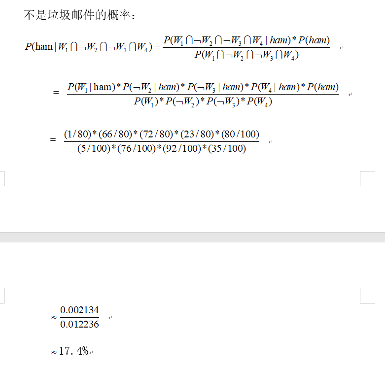

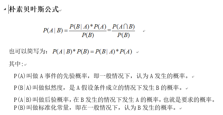
案例:邮件分类预测:是否垃圾邮件

sms_spam.txt

type,text
ham,00 008704050406 008704050406 008704050406 008704050406 00 00 00 00 00 00 Hope Hope Hope you are having a good week. Just checking in
ham,K..give back my thanks.
ham,Am also doing in cbe only. But have to pay.
spam,"complimentary 4 STAR Ibiza Holiday or £10,000 cash needs your URGENT collection. 09066364349 NOW from Landline not to lose out! Box434SK38WP150PPM18+"
spam,okmail: Dear Dave this is your final notice to collect your 4* Tenerife Holiday or #5000 CASH award! Call 09061743806 from landline. TCs SAE Box326 CW25WX 150ppm
ham,Aiya we discuss later lar... Pick u up at 4 is it?
ham,Are you this much buzy
ham,Please ask mummy to call father
spam,Marvel Mobile Play the official Ultimate Spider-man game (£4.50) on ur mobile right now. Text SPIDER to 83338 for the game & we ll send u a FREE 8Ball wallpaper
ham,"fyi I'm at usf now, swing by the room whenever"
ham,"Sure thing big man. i have hockey elections at 6, shouldn€˜t go on longer than an hour though"
ham,I anything lor...
ham,"By march ending, i should be ready. But will call you for sure. The problem is that my capital never complete. How far with you. How's work and the ladies"
ham,"Hmm well, night night "
ham,K I'll be sure to get up before noon and see what's what
ham,Ha ha cool cool chikku chikku:-):-DB-)


bayes.py

# coding:utf-8

import os
import sys
#codecs 编码转换模块
import codecs

# 讲训练样本中的中文文章分词并存入文本文件中

# if __name__ == '__main__':
#     corpus = []
#     f = codecs.open("D:/workspaceR/news_spam.csv", "r", "utf-8")
#     f1 = codecs.open("D:/workspaceR/news_spam_jieba.csv", "w", "utf-8")
#     count = 0
#     while True:
#         line = f.readline()
#         if line:
#             count = count + 1
#             line = line.split(",")
#             s = line[1]
#             words=pseg.cut(s)
#             temp = []
#             for key in words:
#                 temp.append(key.word)
#             sentence = " ".join(temp)
#             print line[0],',',sentence
#             corpus.append(sentence)
#             f1.write(line[0])
#             f1.write(',')
#             f1.write(sentence)
#             f1.write('
')
#         else:
#             break
#     f.close()
#     f1.close()


######################################################
#Multinomial Naive Bayes Classifier
print '*************************
Naive Bayes
*************************'
from sklearn.naive_bayes import MultinomialNB
from sklearn.feature_extraction.text import CountVectorizer

if __name__ == '__main__':
    # 读取文本构建语料库
    corpus = []
    labels = []
    corpus_test = []
    labels_test = []
    f = codecs.open("./sms_spam.txt", "rb")
    count = 0
    while True:
        #readline() 方法用于从文件读取整行,包括 "
" 字符。
        line = f.readline()
        #读取第一行,第一行数据是列头,不统计
        if count == 0:
            count = count + 1
            continue
        if line:
            count = count + 1
            line = line.split(",")
            label = line[0]
            sentence = line[1]
            corpus.append(sentence)
            if "ham"==label:
                labels.append(0)
            elif "spam"==label:
                labels.append(1)
            if count > 5550:
                corpus_test.append(sentence)
                if "ham"==label:
                    labels_test.append(0)
                elif "spam"==label:
                    labels_test.append(1)
        else:
            break
    # 文本特征提取:
    #     将文本数据转化成特征向量的过程
    #     比较常用的文本特征表示法为词袋法
    #
    # 词袋法:
    #     不考虑词语出现的顺序,每个出现过的词汇单独作为一列特征
    #     这些不重复的特征词汇集合为词表
    #     每一个文本都可以在很长的词表上统计出一个很多列的特征向量
    #CountVectorizer是将文本向量转换成稀疏表示数值向量(字符频率向量)  vectorizer 将文档词块化,只考虑词汇在文本中出现的频率
    #词袋
    vectorizer=CountVectorizer()
    #每行的词向量,fea_train是一个矩阵
    fea_train = vectorizer.fit_transform(corpus)

    print "vectorizer.get_feature_names is ",vectorizer.get_feature_names()
    print "fea_train is ",fea_train.toarray()

    #vocabulary=vectorizer.vocabulary_ 只计算上面vectorizer中单词的tf(term frequency 词频)
    vectorizer2=CountVectorizer(vocabulary=vectorizer.vocabulary_)
    fea_test = vectorizer2.fit_transform(corpus_test)
#     print vectorizer2.get_feature_names()
#     print fea_test.toarray()

    #create the Multinomial Naive Bayesian Classifier
    #alpha = 1 拉普拉斯估计给每个单词个数加1
    clf = MultinomialNB(alpha = 1)
    clf.fit(fea_train,labels)

    pred = clf.predict(fea_test);
    for p in pred:
        if p == 0:
            print "正常邮件"
        else:
            print "垃圾邮件"


scala 代码

sample_naive_bayes_data.txt   ## 相当于上边python代码的sentence 编码化。
label word0出现次 wor1 0次, word2 0次
0,1 0 0
0,2 0 0
0,3 0 0
0,4 0 0
1,0 1 0
1,0 2 0
1,0 3 0
1,0 4 0
2,0 0 1
2,0 0 2
2,0 0 3
2,0 0 4

Naive_bayes.scala
package com.bjsxt.bayes

import org.apache.spark.{ SparkConf, SparkContext }
import org.apache.spark.mllib.classification.{ NaiveBayes, NaiveBayesModel }
import org.apache.spark.mllib.linalg.Vectors
import org.apache.spark.mllib.regression.LabeledPoint

object Naive_bayes {
  def main(args: Array[String]) {
    //1 构建Spark对象
    val conf = new SparkConf().setAppName("Naive_bayes").setMaster("local")
    val sc = new SparkContext(conf)
    //读取样本数据1
    val data = sc.textFile("./sample_naive_bayes_data.txt")
    val parsedData = data.map { line =>
      val parts = line.split(',')
      LabeledPoint(parts(0).toDouble, Vectors.dense(parts(1).split(' ').map(_.toDouble)))
    }

    //样本数据划分训练样本与测试样本
    val splits = parsedData.randomSplit(Array(0.5, 0.5), seed = 11L)
    val training = splits(0)
    val test = splits(1)

    //新建贝叶斯分类模型模型,并训练 ,lambda 拉普拉斯估计
    val model = NaiveBayes.train(training, lambda = 1.0)

    //对测试样本进行测试
    val predictionAndLabel = test.map(p => (model.predict(p.features), p.label))
    val print_predict = predictionAndLabel.take(100)
    println("prediction" + "	" + "label")
    for (i <- 0 to print_predict.length - 1) {
      println(print_predict(i)._1 + "	" + print_predict(i)._2)
    }

    val accuracy = 1.0 * predictionAndLabel.filter(x => x._1 == x._2).count() / test.count()
    println(accuracy)
    val result = model.predict(Vectors.dense(Array[Double](80,0,0)))
    println("result = "+result)
    //保存模型
//    val ModelPath = "./naive_bayes_model"
//    model.save(sc, ModelPath)
//    val sameModel = NaiveBayesModel.load(sc, ModelPath)

  }
}


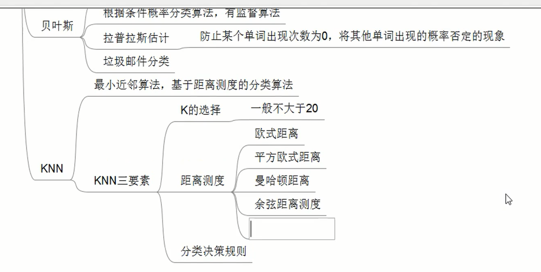
例子
datingTestSet2.txt
40920 8.326976 0.953952 3
14488 7.153469 1.673904 2
26052 1.441871 0.805124 1
75136 13.147394 0.428964 1
38344 1.669788 0.134296 1
72993 10.141740 1.032955 1
35948 6.830792 1.213192 3
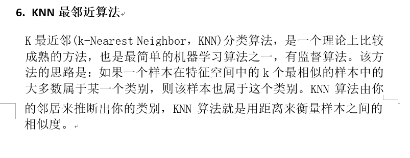
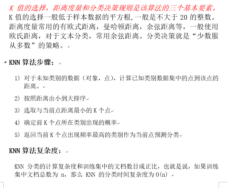
KNNDateOnHand.py
#coding:utf-8
import numpy as np
import operator
#matplotlib 绘图模块
import matplotlib.pyplot as plt
# from array import array
# from matplotlib.font_manager import FontProperties
#normData 测试数据集的某行, dataSet 训练数据集 ,labels 训练数据集的类别,k k的值
def classify(normData,dataSet,labels,k):
#计算行数
dataSetSize = dataSet.shape[0]
# print ('dataSetSize 长度 =%d'%dataSetSize)
#当前点到所有点的坐标差值 ,np.tile(x,(y,1)) 复制x 共y行 1列
diffMat = np.tile(normData, (dataSetSize,1)) - dataSet
#对每个坐标差值平方
sqDiffMat = diffMat ** 2
#对于二维数组 sqDiffMat.sum(axis=0)指 对向量每列求和,sqDiffMat.sum(axis=1)是对向量每行求和,返回一个长度为行数的数组
#例如:narr = array([[ 1., 4., 6.],
# [ 2., 5., 3.]])
# narr.sum(axis=1) = array([ 11., 10.])
# narr.sum(axis=0) = array([ 3., 9., 9.])
sqDistances = sqDiffMat.sum(axis = 1)
#欧式距离 最后开方
distance = sqDistances ** 0.5
#x.argsort() 将x中的元素从小到大排序,提取其对应的index 索引,返回数组
#例: tsum = array([ 11., 10.]) ---- tsum.argsort() = array([1, 0])
sortedDistIndicies = distance.argsort()
# classCount保存的K是魅力类型 V:在K个近邻中某一个类型的次数
classCount = {}
for i in range(k):
#获取对应的下标的类别
voteLabel = labels[sortedDistIndicies[i]]
#给相同的类别次数计数
classCount[voteLabel] = classCount.get(voteLabel,0) + 1
#sorted 排序 返回新的list
# sortedClassCount = sorted(classCount.items(),key=operator.itemgetter(1),reverse=True)
sortedClassCount = sorted(classCount.items(),key=lambda x:x[1],reverse=True)
return sortedClassCount[0][0]
def file2matrix(filename):
fr = open(filename)
#readlines:是一次性将这个文本的内容全部加载到内存中(列表)
arrayOflines = fr.readlines()
numOfLines = len(arrayOflines)
# print "numOfLines = " , numOfLines
#numpy.zeros 创建给定类型的数组 numOfLines 行 ,3列
returnMat = np.zeros((numOfLines,3))
#存结果的列表
classLabelVector = []
index = 0
for line in arrayOflines:
#去掉一行的头尾空格
line = line.strip()
listFromline = line.split(' ')
returnMat[index,:] = listFromline[0:3]
classLabelVector.append(int(listFromline[-1]))
index += 1
return returnMat,classLabelVector
'''
将训练集中的数据进行归一化
归一化的目的:
训练集中飞行公里数这一维度中的值是非常大,那么这个纬度值对于最终的计算结果(两点的距离)影响是非常大,
远远超过其他的两个维度对于最终结果的影响
实际约会姑娘认为这三个特征是同等重要的
下面使用最大最小值归一化的方式将训练集中的数据进行归一化
'''
#将数据归一化
def autoNorm(dataSet):
# dataSet.min(0) 代表的是统计这个矩阵中每一列的最小值 返回值是一个矩阵1*3矩阵
#例如: numpyarray = array([[1,4,6],
# [2,5,3]])
# numpyarray.min(0) = array([1,4,3]) numpyarray.min(1) = array([1,2])
# numpyarray.max(0) = array([2,5,6]) numpyarray.max(1) = array([6,5])
minVals = dataSet.min(0)
maxVals = dataSet.max(0)
ranges = maxVals - minVals
#dataSet.shape[0] 计算行数, shape[1] 计算列数
m = dataSet.shape[0]
# print '行数 = %d' %(m)
# print maxVals
# normDataSet存储归一化后的数据
# normDataSet = np.zeros(np.shape(dataSet))
#np.tile(minVals,(m,1)) 在行的方向上重复 minVals m次 即复制m行,在列的方向上重复munVals 1次,即复制1列
normDataSet = dataSet - np.tile(minVals,(m,1))
normDataSet = normDataSet / np.tile(ranges,(m,1))
return normDataSet,ranges,minVals
def datingClassTest():
hoRatio = 0.1
datingDataMat,datingLabels = file2matrix('./datingTestSet2.txt')
#将数据归一化
normMat,ranges,minVals = autoNorm(datingDataMat)
# m 是 : normMat行数 = 1000
m = normMat.shape[0]
# print 'm =%d 行'%m
#取出100行数据测试
numTestVecs = int(m*hoRatio)
errorCount = 0.0
for i in range(numTestVecs):
#normMat[i,:] 取出数据的第i行,normMat[numTestVecs:m,:]取出数据中的100行到1000行 作为训练集,datingLabels[numTestVecs:m] 取出数据中100行到1000行的类别,4是K
classifierResult = classify(normMat[i,:],normMat[numTestVecs:m,:],datingLabels[numTestVecs:m],4)
print('模型预测值: %d ,真实值 : %d' %(classifierResult,datingLabels[i]))
if (classifierResult != datingLabels[i]):
errorCount += 1.0
errorRate = errorCount / float(numTestVecs)
print '正确率 : %f' %(1-errorRate)
return 1-errorRate
'''
拿到每条样本的飞行里程数和玩视频游戏所消耗的时间百分比这两个维度的值,使用散点图
'''
def createScatterDiagram():
datingDataMat,datingLabels = file2matrix('datingTestSet2.txt')
type1_x = []
type1_y = []
type2_x = []
type2_y = []
type3_x = []
type3_y = []
#生成一个新的图像
fig = plt.figure()
#matplotlib下, 一个 Figure 对象可以包含多个子图(Axes), 可以使用 subplot() 快速绘制
#subplot(numRows, numCols, plotNum)图表的整个绘图区域被分成 numRows 行和 numCols 列,按照从左到右,从上到下的顺序对每个子区域进行编号,左上的子区域的编号为1
#plt.subplot(111)等价于plt.subplot(1,1,1)
axes = plt.subplot(111)
#设置字体 黑体 ,用来正常显示中文标签
plt.rcParams['font.sans-serif']=['SimHei']
for i in range(len(datingLabels)):
if datingLabels[i] == 1: # 不喜欢
type1_x.append(datingDataMat[i][0])
type1_y.append(datingDataMat[i][1])
if datingLabels[i] == 2: # 魅力一般
type2_x.append(datingDataMat[i][0])
type2_y.append(datingDataMat[i][1])
if datingLabels[i] == 3: # 极具魅力
type3_x.append(datingDataMat[i][0])
type3_y.append(datingDataMat[i][1])
#绘制散点图 ,前两个参数表示相同长度的数组序列 ,s 表示点的大小, c表示颜色
type1 = axes.scatter(type1_x, type1_y, s=20, c='red')
type2 = axes.scatter(type2_x, type2_y, s=40, c='green')
type3 = axes.scatter(type3_x, type3_y, s=50, c='blue')
plt.title(u'标题')
plt.xlabel(u'每年飞行里程数')
plt.ylabel(u'玩视频游戏所消耗的时间百分比')
#loc 设置图例的位置 2是upper left
axes.legend((type1, type2, type3), (u'不喜欢', u'魅力一般', u'极具魅力'), loc=2)
# plt.scatter(datingDataMat[:,0],datingDataMat[:,1],c = datingLabels)
plt.show()
def classifyperson():
resultList = ['没感觉', '看起来还行','极具魅力']
input_man= [30000,3,0.1]
# input_man= [13963,0.000000,1.437030]
datingDataMat,datingLabels = file2matrix('datingTestSet2.txt')
normMat,ranges,minVals = autoNorm(datingDataMat)
result = classify((input_man - minVals)/ranges,normMat,datingLabels,3)
print ('你即将约会的人是:%s'%resultList[result-1])
if __name__ == '__main__':
# createScatterDiagram观察数据的分布情况
# createScatterDiagram()
acc = datingClassTest()
if(acc > 0.9):
classifyperson()
## 不采用上边的手动实现,调用库实现。
KNNDateByScikit-learn.py

#coding:utf-8

from sklearn.neighbors import NearestNeighbors
import numpy as np
from KNNDateOnHand import *

if __name__ == '__main__':
    datingDataMat,datingLabels = file2matrix('datingTestSet2.txt')
    normMat,ranges,minVals = autoNorm(datingDataMat)
    # n_neighbors=3 表示查找的近邻数,默认是5
    # fit:用normMat作为训练集拟合模型   n_neighbors:几个最近邻
    #NearestNeighbors 默认使用的就是欧式距离测度
    nbrs = NearestNeighbors(n_neighbors=3).fit(normMat)
    input_man= [9289,9.666576,1.370330]
    #数据归一化
    S = (input_man - minVals)/ranges
    #找到当前点的K个临近点,也就是找到临近的3个点
    #indices 返回的距离数据集中最近点的坐标的下标。  distance 返回的是距离数据集中最近点的距离
    distances, indices = nbrs.kneighbors(S)
    print distances
    print indices
    # classCount   K:类别名    V:这个类别中的样本出现的次数
    classCount = {}
    for i in range(3):
        #找出对应的索引的类别号
        voteLabel = datingLabels[indices[0][i]]
        classCount[voteLabel] = classCount.get(voteLabel,0) + 1
    sortedClassCount = sorted(classCount.items(),key=operator.itemgetter(1),reverse=True)
    resultList = ['没感觉', '看起来还行','极具魅力']
    print resultList[sortedClassCount[0][0]-1]
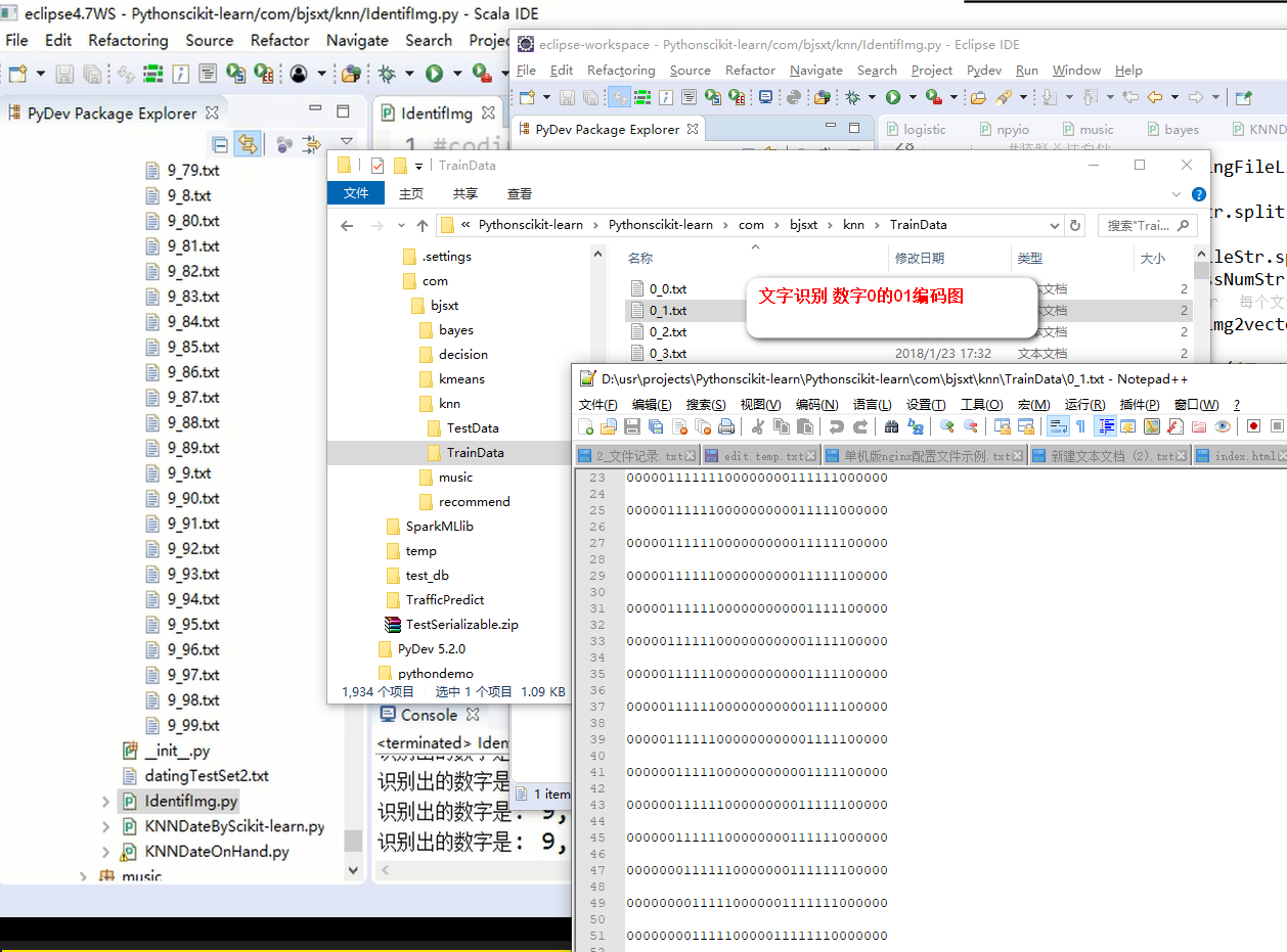
IdentifImg.py

#coding:utf-8

import os
import numpy as np
from KNNDateOnHand import classify

#此方法将每个文件中32*32的矩阵数据,转换到1*1024一行中
def img2vector(filename):
    #创建一个1行1024列的矩阵
    returnVect = np.zeros((1,1024))
    #打开当前的文件
    fr = open(filename)
    #每个文件中有32行,每行有32列数据,遍历32个行,将32个列数据放入1024的列中
    for i in range(32):
        lineStr = fr.readline()
        for j in range(32):
            returnVect[0,32*i+j] = int(lineStr[j])
    return returnVect

def IdentifImgClassTest():
    hwLabels = []
    #读取训练集 TrainData目录下所有的文件和文件夹
    trainingFileList = os.listdir('TrainData')
    m = len(trainingFileList)
    #zeros((m,1024)) 返回一个m行 ,1024列的矩阵,默认是浮点型的
    trainingMat = np.zeros((m,1024))
    for i in range(m):
        #获取文件名称
        fileNameStr = trainingFileList[i]
        #获取文件除了后缀的名称
        fileStr = fileNameStr.split('.')[0]
        #获取文件"数字"的类别
        classNumStr = int(fileStr.split('_')[0])
        hwLabels.append(classNumStr)
        #构建训练集, img2vector  每个文件返回一行数据 1024列
        trainingMat[i,:] = img2vector('TrainData/%s' % fileNameStr)
    #读取测试集数据
    testFileList = os.listdir('TestData')
    errorCount = 0.0
    mTest = len(testFileList)
    for i in range(mTest):
        fileNameStr = testFileList[i]
        fileStr = fileNameStr.split('.')[0]
        classNumStr = int(fileStr.split('_')[0])
        vectorUnderTest = img2vector('TestData/%s' % fileNameStr)
        classifierResult = classify(vectorUnderTest, trainingMat, hwLabels, 3)
        print "识别出的数字是: %d, 真实数字是: %d" % (classifierResult, classNumStr)
        if (classifierResult != classNumStr):
            errorCount += 1.0
    print "
识别错误次数 %d" % errorCount
    errorRate = errorCount/float(mTest)
    print "
正确率: %f" % (1-errorRate)

if __name__ == '__main__':
    IdentifImgClassTest()

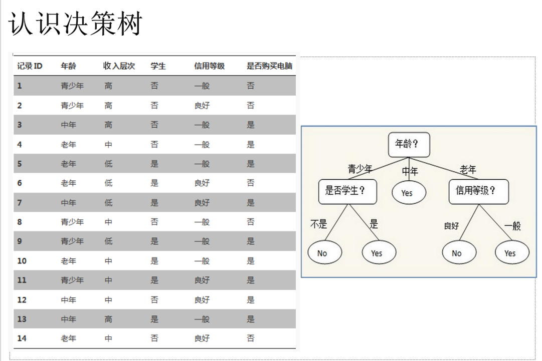
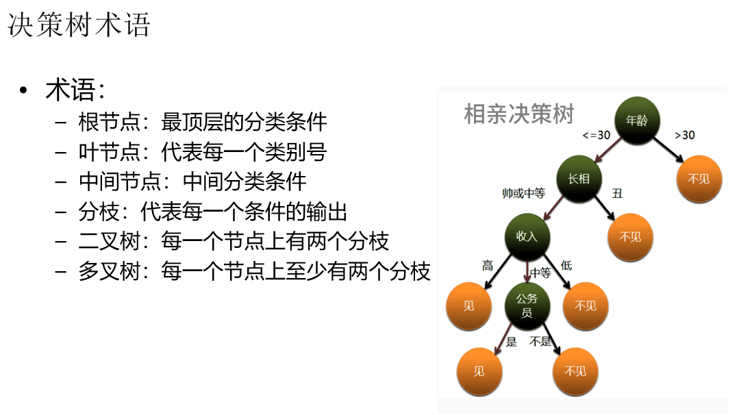
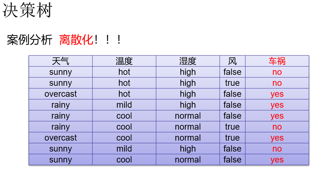


连续数据 分类 形成离散化数据, 决策树的数据一定是分类数据


例子:
汽车数据样本.txt
1 1:2 2:1 3:1 4:1 5:80
1 1:3 2:2 3:1 4:1 5:77
1 1:3 2:2 3:1 4:1 5:77
1 1:2 2:1 3:1 4:1 5:77
1 1:2 2:1 3:1 4:1 5:72
1 1:3 2:2 3:1 4:1 5:40
1 1:2 2:2 3:1 4:1 5:61
1 1:2 2:1 3:1 4:1 5:69
1 1:2 2:1 3:1 4:1 5:71
1 1:3 2:2 3:1 4:1 5:76
1 1:2 2:1 3:1 4:1 5:74
1 1:2 2:1 3:1 4:1 5:80
1 1:3 2:1 3:1 4:1 5:61
1 1:2 2:1 3:1 4:1 5:68
1 1:2 2:2 3:1 4:1 5:79
1 1:3 2:1 3:1 4:1 5:73
ClassificationDecisionTree.scala
package com.bjsxt.rf
import org.apache.spark.mllib.tree.DecisionTree
import org.apache.spark.mllib.util.MLUtils
import org.apache.spark.{SparkContext, SparkConf}
/**
* 决策树
*/
object ClassificationDecisionTree {
def main(args: Array[String]): Unit = {
val conf = new SparkConf()
conf.setAppName("analysItem")
conf.setMaster("local[3]")
val sc = new SparkContext(conf)
val data = MLUtils.loadLibSVMFile(sc, "汽车数据样本.txt")
// Split the data into training and test sets (30% held out for testing)
val splits = data.randomSplit(Array(0.7, 0.3))
val (trainingData, testData) = (splits(0), splits(1))
//指明分类的类别
val numClasses=2
//指定离散变量,未指明的都当作连续变量处理
//某列下有1,2,3类别 处理时候要自定为4类,虽然没有0,但是程序默认从0开始分类
//这里天气维度有3类,但是要指明4,这里是个坑,后面以此类推
val categoricalFeaturesInfo=Map[Int,Int](0->4,1->4,2->3,3->3)
//设定评判标准 "gini"/"entropy"
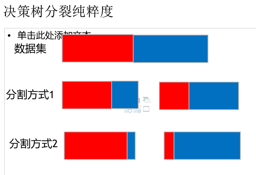
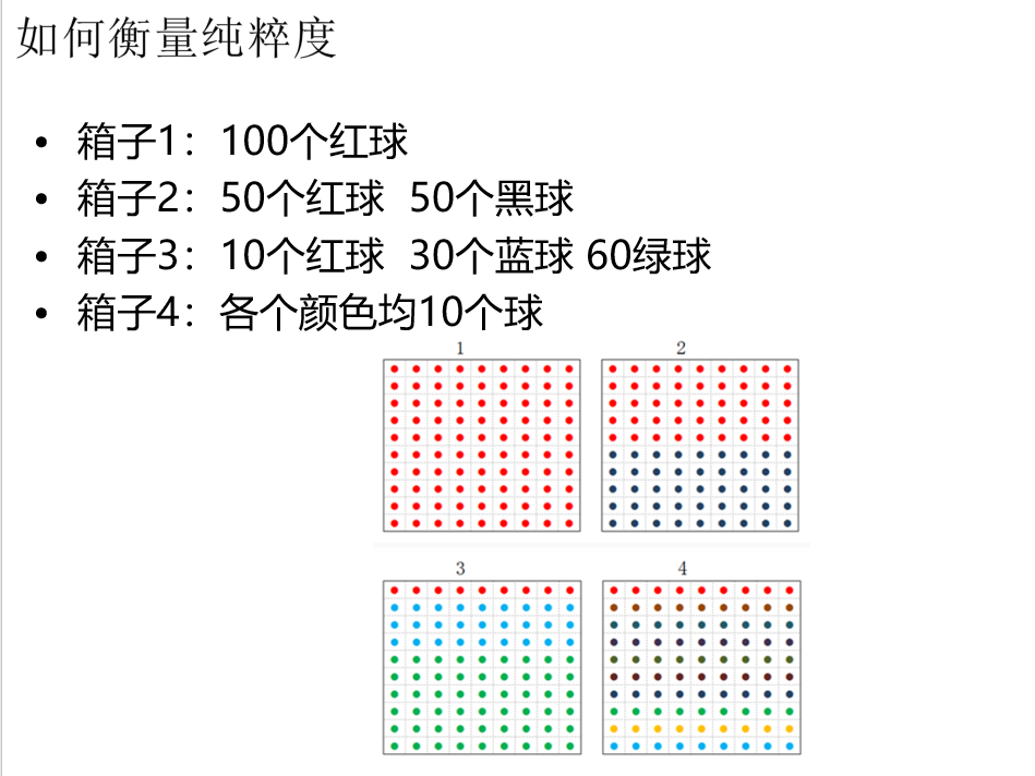
val impurity="entropy"
//树的最大深度,太深运算量大也没有必要 剪枝 防止模型的过拟合!!!
val maxDepth=3
//设置离散化程度,连续数据需要离散化,分成32个区间,默认其实就是32,分割的区间保证数量差不多 这个参数也可以进行剪枝
val maxBins=32
//生成模型
val model =DecisionTree.trainClassifier(trainingData,numClasses,categoricalFeaturesInfo,impurity,maxDepth,maxBins)
//测试
val labelAndPreds = testData.map { point =>
val prediction = model.predict(point.features)
(point.label, prediction)
}
val testErr = labelAndPreds.filter(r => r._1 != r._2).count().toDouble / testData.count()
println("Test Error = " + testErr)
println("Learned classification tree model:
" + model.toDebugString)
}
}

ClassificationRandomForest.scala

package com.bjsxt.rf

import org.apache.spark.{SparkContext, SparkConf}
import org.apache.spark.mllib.util.MLUtils
import org.apache.spark.mllib.tree.RandomForest
/**
 * 随机森林
 *
 */
object ClassificationRandomForest {
  def main(args: Array[String]): Unit = {
	  val conf = new SparkConf()
			  conf.setAppName("analysItem")
			  conf.setMaster("local[3]")
			  val sc = new SparkContext(conf)
    //读取数据
    val data =  MLUtils.loadLibSVMFile(sc,"汽车数据样本.txt")
    //将样本按7:3的比例分成
    val splits = data.randomSplit(Array(0.7, 0.3))
    val (trainingData, testData) = (splits(0), splits(1))
    //分类数
    val numClasses = 2
    // categoricalFeaturesInfo 为空,意味着所有的特征为连续型变量
    val categoricalFeaturesInfo =Map[Int, Int](0->4,1->4,2->3,3->3)
    //树的个数
    val numTrees = 3
    //特征子集采样策略,auto 表示算法自主选取
    //"auto"根据特征数量在4个中进行选择
    // 1:all 全部特征 。2:sqrt 把特征数量开根号后随机选择的 。 3:log2 取对数个。 4:onethird 三分之一
    val featureSubsetStrategy = "auto"
    //纯度计算  "gini"/"entropy"
    val impurity = "entropy"
    //树的最大层次
    val maxDepth = 3
    //特征最大装箱数,即连续数据离散化的区间
    val maxBins = 32
    //训练随机森林分类器,trainClassifier 返回的是 RandomForestModel 对象
    val model = RandomForest.trainClassifier(trainingData, numClasses, categoricalFeaturesInfo,
      numTrees, featureSubsetStrategy, impurity, maxDepth, maxBins)
    //打印模型
    println(model.toDebugString)
    //保存模型
   //model.save(sc,"汽车保险")
    //在测试集上进行测试
    val count = testData.map { point =>
        val prediction = model.predict(point.features)
    //    Math.abs(prediction-point.label)
        (prediction,point.label)
     }.filter(r => r._1 != r._2).count()
    println("Test Error = " + count.toDouble/testData.count().toDouble)
    println("model "+model.toDebugString)
  }
}
mean
英 [miːn]   美 [miːn]
v.
表示…的意思;意思是;本意是;打算;意欲;有…的目的
adj.
吝啬的;小气的;不善良;刻薄;要发怒的;要发狂的
n.
中间;中庸;折中;平均数;平均值;算术中项

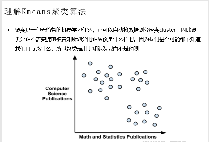
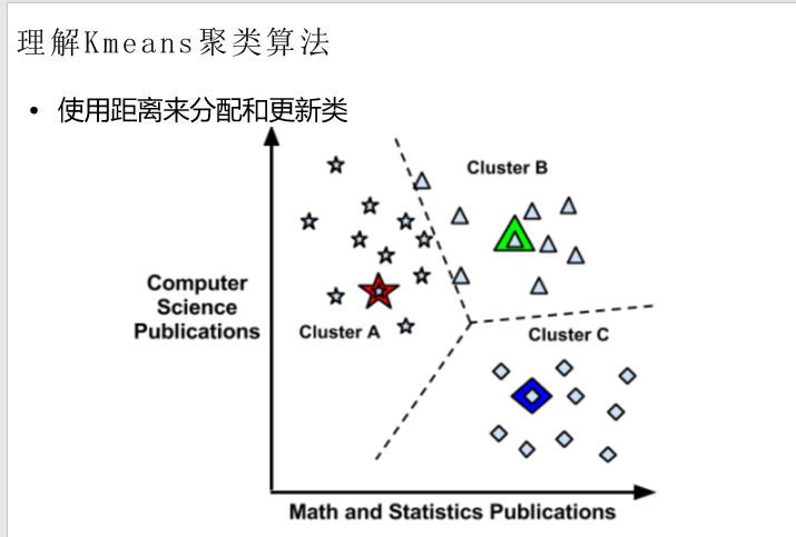
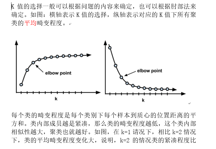
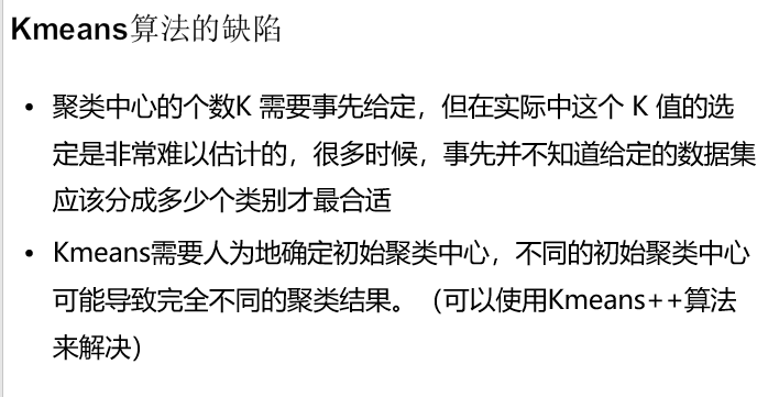
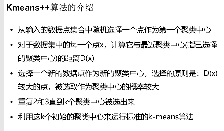
testSet.txt

1.658985	4.285136

-3.453687	3.424321

4.838138	-1.151539

-5.379713	-3.362104

0.972564	2.924086

-3.567919	1.531611

0.450614	-3.302219

-3.487105	-1.724432

2.668759	1.594842

-3.156485	3.191137

KMeansOnHand.py

# encoding:utf-8

import numpy as np


#将每行数据放入一个数组内列表,返回一个二维列表
def loadDataSet(fileName):
    #创建空列表
    dataMat = []
    fr = open(fileName)
    for line in fr.readlines():
        #按照制表符切割每行,返回一个列表list
        curLine = line.strip().split('	')
        #将切分后的每个列表中的元素,以float形式返回,map()内置函数,返回一个list
        fltLine = map(float,curLine)
        dataMat.append(fltLine)
    return dataMat

#两点欧式距离
def distEclud(vecA, vecB):
    #np.power(x1,x2)  对x1中的每个元素求x2次方,不会改变x1。
    return np.sqrt(np.sum(np.power(vecA - vecB, 2)))

#随机找到3个中心点的位置坐标,返回一个3*2的矩阵
def randCent(dataSet, k):
    #返回dataSet列数,2列
    n = np.shape(dataSet)[1]
    '''
        centroids是一个3*2的矩阵,用于存储三个中心点的坐标
    '''
    centroids = np.mat(np.zeros((k,n)))
    for j in range(n):
        #统计每一列的最小值
        minJ = min(dataSet[:,j])
        #每列最大值与最小值的差值
        rangeJ = float(max(dataSet[:,j]) - minJ)
        #np.random.rand(k,1) 产生k行1列的数组,里面的数据是0~1的浮点型 随机数。
        array2 = minJ + rangeJ * np.random.rand(k,1)
        #转换成k*1矩阵 赋值给centroids
        centroids[:,j] = np.mat(array2)
    return centroids


def kMeans(dataSet, k, distMeas=distEclud, createCent=randCent):
    #计算矩阵所有 行数  m=80
    m = np.shape(dataSet)[0]
    #zeros((m,2)) 创建一个80行,2列的二维数组
    #numpy.mat 将二维数组转换成矩阵
    clusterAssment = np.mat(np.zeros((m,2)))

    #createCent找到K个随机中心点坐标
    centroids = createCent(dataSet, k)
#     print centroids
    clusterChanged = True
    while clusterChanged:
        clusterChanged = False
        #遍历80个数据到每个中心点的距离
        for i in range(m):
            #np.inf float的最大值,无穷大
            minDist = np.inf
            #当前点属于的类别号
            minIndex = -1
            #每个样本点到三个中心点的距离
            for j in range(k):
#                 x = centroids[j,:]
#                 print x
                #返回两点距离的值
                distJI = distMeas(centroids[j,:],dataSet[i,:])
                if distJI < minDist:
                    #当前最小距离的值
                    minDist = distJI
                    #当前最小值属于哪个聚类
                    minIndex = j
            #有与上次迭代计算的当前点的类别不相同的点
            if clusterAssment[i,0] != minIndex:
                clusterChanged = True
            #将当前点的类别号和最小距离 赋值给clusterAssment的一行
            clusterAssment[i,:] = minIndex,minDist
        for cent in range(k):
#             array = clusterAssment[:,0].A==cent
#             result = np.nonzero(clusterAssment[:,0].A==cent)[0]
            #clusterAssment[:,0].A 将0列 也就是类别号转换成数组
            #clusterAssment[:,0].A==cent 返回的是一列,列中各个元素是 True或者False,True代表的是当前遍历的cent类别
            #np.nonzero(clusterAssment[:,0].A==cent)  返回数组中值不为False的元素对应的行号下标数组 和列号下标数组
            #ptsInClust 取出的是对应是当前遍历cent类别的 所有行数据组成的一个矩阵
            ptsInClust = dataSet[np.nonzero(clusterAssment[:,0].A==cent)[0]]
            #numpy.mean 计算矩阵的均值,axis=0计算每列的均值,axis=1计算每行的均值。
            #这里是每经过一次while计算都会重新找到各个类别中中心点坐标的位置  ,axis = 0 是各个列求均值
            centroids[cent,:] = np.mean(ptsInClust, axis=0)
    #返回 【 当前三个中心点的坐标】 【每个点的类别号,和到当前中心点的最小距离】
    return centroids, clusterAssment

if __name__ == '__main__':
    #numpy.mat 将数据转换成80*2的矩阵
    dataMat = np.mat(loadDataSet('./testSet.txt'))
    k=3
    #centroids 三个中心点的坐标。clusterAssment 每个点的类别号|到当前中心点的最小距离
    centroids, clusterAssment = kMeans(dataMat, k, distMeas=distEclud, createCent=randCent)
    print centroids
    print clusterAssment
KMeansByScikitlearn.py  ## 带图

#coding:utf-8
import numpy as np
import matplotlib.pyplot as plt
from sklearn.cluster import KMeans
from sklearn.datasets import make_blobs

#建立12*12英寸  新的图像
plt.figure(figsize=(12, 12))
n_samples = 1500
random_state = 170
'''
    make_blobs函数是为聚类产生数据集 , 产生一个数据集和相应的标签
        n_samples:表示数据样本点个数,默认值100
        n_features:表示数据的维度,特征,默认值是2
        centers:产生数据的中心点,默认值3个
        shuffle :洗乱,默认值是True
        random_state:官网解释是随机生成器的种子
'''
#x返回的是向量化的数据点,y返回的是对应数据的类别号
x,y = make_blobs(n_samples=n_samples, random_state=random_state)
print 'x=',x,type(x),'y=',y
#使用KMeans去聚类,返回聚好的类别集合, n_clusters聚合成几类
y_pred = KMeans(n_clusters=3, random_state=random_state).fit_predict(x)
print "y_pred : ",y_pred
#subplot 绘制多个子图,221 等价于2,2,1 表示两行两列的子图中的第一个
plt.subplot(221)
#scatter 绘制散点图   ,c 指定颜色
plt.scatter(x[:, 0], x[:, 1], c=y_pred)
plt.title("kmeans01")


transformation = [[ 0.60834549, -0.63667341], [-0.40887718, 0.85253229]]
#numpy.dot 矩阵相乘
#a1= [[1,2]
#     [3,4]
#     [5,6]]
#a2= [[10,20]
#     [30,40]]
#a1*a2 = [[1*10+2*30,1*20+2*40]
#         [3*10+4*30,3*20+4*40]
#         [5*10+5*30,6*20+6*40]
#            ]
X_aniso = np.dot(x, transformation)
y_pred = KMeans(n_clusters=3, random_state=random_state).fit_predict(X_aniso)
plt.subplot(222)
plt.scatter(X_aniso[:, 0], X_aniso[:, 1], c=y_pred)
plt.title("kmeans02")


#vstack 是合并矩阵,将y=0类别的取出500行,y=1类别的取出100行,y=2类别的取出10行
X_filtered = np.vstack((x[y == 0][:500], x[y == 1][:100], x[y == 2][:10]))
y_pred = KMeans(n_clusters=3, random_state=random_state).fit_predict(X_filtered)
plt.subplot(223)
plt.scatter(X_filtered[:, 0], X_filtered[:, 1], c=y_pred)
plt.title("kmeans03")


dataMat = []
fr = open("testSet.txt","r")
for line in fr.readlines():
    if line.strip() <> "":
        curLine = line.strip().split('	')
        fltLine = map(float,curLine)
        dataMat.append(fltLine)
dataMat = np.array(dataMat)
#调用Scikitlearn中的KMeans
#KMeans 中参数 init='k-means++' 默认就是k-means++  如果设置为'random'是随机找中心点
y_pred = KMeans(n_clusters=4).fit_predict(dataMat)
plt.subplot(224)
plt.scatter(dataMat[:,0], dataMat[:, 1], c=y_pred)
plt.title("kmeans04")
plt.savefig("./kmeans.png")
plt.show()
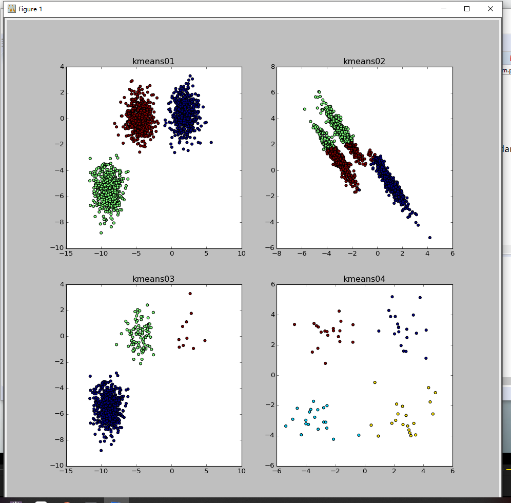
kmeans_data.txt

0.0 0.0 0.0
0.1 0.1 0.1
0.2 0.2 0.2
9.0 9.0 9.0
9.1 9.1 9.1
9.2 9.2 9.2

KMeansScala.scala

package com.bjsxt.kmeans

import scala.tools.scalap.Main
import org.apache.spark.SparkConf
import org.apache.spark.SparkContext
import org.apache.spark.sql.SQLContext
import org.apache.spark.mllib.clustering.KMeansModel
import org.apache.spark.mllib.clustering.KMeans
import org.apache.spark.mllib.linalg.Vectors
/**
 * 通过数据集使用kmeans训练模型
 */
object KMeansScala {
  def main(args: Array[String]): Unit = {

    //1 构建Spark对象
    val conf = new SparkConf().setAppName("KMeans").setMaster("local")
    val sc = new SparkContext(conf)

    // 读取样本数据1,格式为LIBSVM format
    val data = sc.textFile("kmeans_data.txt")
    val parsedData = data.map(s => Vectors.dense(s.split(' ').map(_.toDouble))).cache()


    val numClusters = 4  // // 根据原始数据建议分两类,
    val numIterations = 100
    val model = new KMeans().
      //设置聚类的类数
      setK(numClusters).
      //设置找中心点最大的迭代次数
      setMaxIterations(numIterations).
      run(parsedData)

    //四个中心点的坐标
    val centers = model.clusterCenters
    val k = model.k
    centers.foreach(println)
    println(k)
    //保存模型
    model.save(sc, "./Kmeans_model")
    //加载模型
    val sameModel = KMeansModel.load(sc, "./Kmeans_model")
    println(sameModel.predict(Vectors.dense(1,1,1)))


    //SparkSQL读取显示4个中心点坐标
    val sqlContext = new SQLContext(sc)
    sqlContext.read.parquet("./Kmeans_model/data").show()


  }
}

KMeans2.scala

package com.bjsxt.kmeans

import org.apache.spark.SparkConf
import org.apache.spark.SparkContext
import org.apache.spark.mllib.clustering.KMeansModel
import org.apache.spark.mllib.linalg.Vectors
import org.apache.spark.mllib.linalg.Vector

/**
 * 给kmeans指定中心点的位置
 */
object KMeans2 {

  def main(args: Array[String]) {
    val conf = new SparkConf().setAppName("KMeans2").setMaster("local")
    val sc = new SparkContext(conf)

    val rdd = sc.parallelize(List(
      Vectors.dense(Array(-0.1, 0.0, 0.0)),
      Vectors.dense(Array(9.0, 9.0, 9.0)),
      Vectors.dense(Array(3.0, 2.0, 1.0))))

    //指定文件 kmeans_data.txt 中的六个点为中心点坐标。
    val centroids: Array[Vector] = sc.textFile("kmeans_data.txt")
        .map(_.split(" ").map(_.toDouble))
        .map(Vectors.dense(_))
        .collect()


    val model = new KMeansModel(clusterCenters=centroids)
    println("聚类个数 = "+model.k)
    //模型中心点
    model.clusterCenters.foreach { println }
    //预测指定的三条数据
    val result = model.predict(rdd)
    result.collect().foreach(println(_))
  }
}
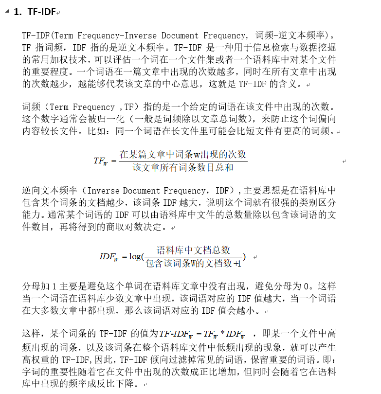
微博案例
IK分词器配置,以及配置外部词典
ext.dic
stopword.dic
IKAnalyzer.cfg.xml
<?xml version="1.0" encoding="UTF-8"?>
<!DOCTYPE properties SYSTEM "http://java.sun.com/dtd/properties.dtd">
<properties>
<comment>IK Analyzer extra configuration</comment>
<!-- configure your own dic here -->
<entry key="ext_dict">ext.dic;</entry>
<!-- configure your own stop dic here -->
<entry key="ext_stopwords">stopword.dic</entry>
</properties>


testdata.txt

3794020835114249	九阳必须是其中之一的其中之一日出
3794020835114250	我要天天和当家看日出
3794020835114251	我要天天和当家看日出

test.scala

package com.bjsxt.kmeans

import scala.collection.mutable.ArrayBuffer
import scala.collection.mutable.ListBuffer

import org.apache.lucene.analysis.TokenStream
import org.apache.lucene.analysis.tokenattributes.CharTermAttribute
import org.apache.spark.SparkConf
import org.apache.spark.SparkContext
import org.apache.spark.mllib.clustering.KMeans
import org.apache.spark.mllib.clustering.KMeansModel
import org.apache.spark.mllib.feature.HashingTF
import org.apache.spark.mllib.feature.IDF
import org.apache.spark.mllib.linalg.Vector
import org.apache.spark.rdd.RDD
import org.wltea.analyzer.lucene.IKAnalyzer
import org.apache.spark.mllib.feature.IDFModel

object test {
  def main(args: Array[String]) {
    val conf = new SparkConf().setAppName("KMeans1").setMaster("local[*]")
    val sc = new SparkContext(conf)
    sc.setLogLevel("WARN")
    val rdd = sc.textFile("./testdata.txt")
    /**
     * wordRDD 是一个KV格式的RDD
     * 	K:微博ID
     * 	V:微博内容分词后的结果 ArrayBuffer
     */
    var wordRDD = rdd.mapPartitions(iterator => {
      val list = new ListBuffer[(String, ArrayBuffer[String])]
      while (iterator.hasNext) {
        //创建分词对象   IKAnalyzer支持两种分词模式:最细粒度和智能分词模式,如果构造函数参数为false,那么使用最细粒度分词。
        val analyzer = new IKAnalyzer(true)
        val line = iterator.next()
        val textArr = line.split("	")
        val id = textArr(0)
        val text = textArr(1)
        //分词     第一个参数只是标识性,没有实际作用,第二个读取的数据
        val ts : TokenStream = analyzer.tokenStream("", text)
        //得到相应词汇的内容
        val term : CharTermAttribute = ts.getAttribute(classOf[CharTermAttribute])
        //重置分词器,使得tokenstream可以重新返回各个分词
    		ts.reset()
    		val arr = new ArrayBuffer[String]
        //遍历分词数据
        while (ts.incrementToken()) {
          arr.+=(term.toString())
        }

        list.append((id, arr))
        analyzer.close()
      }
      list.iterator
    })
    wordRDD = wordRDD.cache()
    //九阳, 必须, 是, 其中之一, 的
    wordRDD.foreach(println)

    /**
     * HashingTF 使用hash表来存储分词
     * HashingTF 是一个Transformer 转换器,在文本处理中,接收词条的集合然后把这些集合转化成固定长度的特征向量,这个算法在哈希的同时会统计各个词条的词频
     * 1000:只是计算每篇微博中1000个单词的词频   最大似然估计思想
     */
    val hashingTF: HashingTF = new HashingTF(100)

    /**
     * tfRDD
     * K:微博ID
     * V:Vector(tf,tf,tf.....)
     *
     * hashingTF.transform(x._2) 计算分词频数(TF)
     */
    val tfRDD = wordRDD.map(x => {
      (x._1, hashingTF.transform(x._2))
    })
    tfRDD.foreach(println)

    /**
     * 得到IDFModel,要计算每个单词在整个语料库中的IDF
     * IDF是一个 Estimator 评价器,在一个数据集上应用它的fit()方法,产生一个IDFModel。 该IDFModel 接收特征向量(由HashingTF产生)
     * new IDF().fit(tfRDD.map(_._2)) 就是在组织训练这个评价器,让评价器知道语料库中有那些个词块,方便计算IDF
     */
    val idf: IDFModel = new IDF().fit(tfRDD.map(_._2))

    /**
     * K:微博 ID
     * V:每一个单词的TF-IDF值
     * tfIdfs这个RDD中的Vector就是训练模型的训练集
     */
    val tfIdfs: RDD[(String, Vector)] = tfRDD.mapValues(idf.transform(_))
    tfIdfs.foreach(x=>{
        println("tfIdfs = "+x)
    })
    //设置聚类个数
    val kcluster = 20
    val kmeans = new KMeans()
    kmeans.setK(kcluster)
    //使用的是kemans++算法来训练模型  "random"|"k-means||"
    kmeans.setInitializationMode("k-means||")
    //设置最大迭代次数
    kmeans.setMaxIterations(100)
    //训练模型
    val kmeansModel: KMeansModel= kmeans.run(tfIdfs.map(_._2))
    //    kmeansModel.save(sc, "d:/model001")
    //打印模型的20个中心点
    val centers = kmeansModel.clusterCenters
    centers.foreach(println)
//    println(kmeansModel.clusterCenters)

    /**
     * 模型预测
     */
    val modelBroadcast = sc.broadcast(kmeansModel)
    /**
     * predicetionRDD KV格式的RDD
     * 	K:微博ID
     * 	V:分类号
     */
    val predicetionRDD = tfIdfs.mapValues(sample => {
      val model = modelBroadcast.value
      model.predict(sample)
    })
//    predicetionRDD.saveAsTextFile("d:/resultttt")

    /**
     * 总结预测结果
     * tfIdfs2wordsRDD:kv格式的RDD
     * K:微博ID
     * V:二元组(Vector(tfidf1,tfidf2....),ArrayBuffer(word,word,word....))
     */
    val tfIdfs2wordsRDD = tfIdfs.join(wordRDD)
    /**
     * result:KV
     * K:微博ID
     * V:(类别号,(Vector(tfidf1,tfidf2....),ArrayBuffer(word,word,word....)))
     */
    val result = predicetionRDD.join(tfIdfs2wordsRDD)

    /**
     * 查看0号类别中tf-idf比较高的单词,能代表这类的主题
     */
    result
      .filter(x => x._2._1 == 0)
      .flatMap(line => {

        val tfIdfV: Vector = line._2._2._1
        val words: ArrayBuffer[String] = line._2._2._2
        val tfIdfA: Array[Double] = tfIdfV.toArray

        val wordL = new ListBuffer[String]()
        val tfIdfL = new ListBuffer[Double]()
        var index = 0
        for(i <- 0 until tfIdfA.length ;if tfIdfV(i) != 0){
          wordL.+=(words(index))
          tfIdfL.+=(tfIdfA(index))
          index += 1
        }
        println(wordL.length + "===" + tfIdfL.length)
        val list = new ListBuffer[(Double, String)]
        for (i <- 0 until wordL.length) {
          list.append((tfIdfV(i), words(i)))
        }
        list
      }).map(_.swap).reduceByKey(_+_).map(_.swap)
      .sortBy(x => x._1, false)
      .map(_._2)
      .take(30).foreach(println)
    sc.stop()
  }

}


original.txt

3793992720744105	#九阳有礼 无需多滤#陷入被窝温柔乡,起床靠毅力?九阳免滤豆浆机C668SG耀世首发!智能预约免过滤,贴心配置强到飞起,让你再续温柔一小时!真的很需要这款九阳豆浆机,这样就可以和小宝贝多待会!@高海澄知 @历衔枫 @郭河九元
3793993084926422	#谢谢你陪我走过2014#好吧,这一年马上就要过去了,同样这一年有欢笑,有泪水,但更多的还是幸福。虽然我知道我很任性[纠结],但宝宝姐姐老婆还是对我超级好好好好好好[群体围观],希望我明年能乖点,听点话 @九阳 @瑷o詠a国际范
3793993291060111	跨年啦。小伙伴们,新年快乐~[笑哈哈][笑哈哈][笑哈哈]@美的电饭煲官方微博 @美的生活电器 @九阳 @SKG互联网家电 @中国电信湖北客服
3793993588106975	我的胆有0.9斤,我想要3.1斤重的铁釜,有份量才够胆量!九阳Alva0716
3793995102741635	《太上青玄慈悲太乙救苦天尊寶懺》 - 起讚   元始運元  神運元神 �化太一尊    九陽天上布恩綸 手內楊枝 遍灑甘露春   大眾悉朝真 群荷深仁 朵朵擁祥雲 大...  (来自 @头条博客) -  顶礼太上青玄慈悲太乙救苦天尊 http://t.cn/zYwwlSY
3793995370610238	#九阳有礼 无需多滤#新年交好运!有了九阳,让生活免滤无忧!@誰能許诺給我一世柔情 @索心进 @错爱990
3793995484592300	#谢谢你陪我走过2014#2014年将至,希望能中一个好东西来送给我的家人。@九阳 @枫叶红了112
37939954845923011	#谢谢你陪我走过2014#2014年将至,希望能中一个好东西来送给我的家人。@九阳 @枫叶红了112
3793995781905340	免过滤,更顺滑,#九阳有礼 无需多滤# 更多营养更安心!@princess佳妮昂 @木凝眉 @单纯会让人受伤航
3793996277455995	#谢谢你陪我走过2014#2014年将至,希望能中一个好东西来送给我的家人。@九阳 @枫叶红了112
3793996323668014	#谢谢你陪我走过2014#2014年将至,希望能中一个好东西来送给我的家人。@九阳 @枫叶红了112

KMeans11.scala

package com.bjsxt.kmeans

import scala.collection.mutable.ArrayBuffer
import scala.collection.mutable.ListBuffer

import org.apache.lucene.analysis.TokenStream
import org.apache.lucene.analysis.tokenattributes.CharTermAttribute
import org.apache.spark.SparkConf
import org.apache.spark.SparkContext
import org.apache.spark.mllib.clustering.KMeans
import org.apache.spark.mllib.feature.HashingTF
import org.apache.spark.mllib.feature.IDF
import org.apache.spark.mllib.feature.IDFModel
import org.apache.spark.rdd.RDD
import org.wltea.analyzer.lucene.IKAnalyzer
import org.apache.spark.mllib.linalg.Vector
import org.apache.spark.mllib.clustering.KMeansModel

object KMeans11 {

  def main(args: Array[String]) {
    val conf = new SparkConf().setAppName("KMeans1").setMaster("local[*]")
    val sc = new SparkContext(conf)

    val rdd = sc.textFile("./original.txt")
    /**
     * wordRDD 是一个KV格式的RDD
     * 	K:微博ID
     * 	V:微博内容分词后的结果 ArrayBuffer
     */
    var wordRDD = rdd.mapPartitions(iterator => {
      val list = new ListBuffer[(String, ArrayBuffer[String])]
      while (iterator.hasNext) {
        //创建分词对象   IKAnalyzer支持两种分词模式:最细粒度和智能分词模式,如果构造函数参数为false,那么使用最细粒度分词。
        val analyzer = new IKAnalyzer(true)
        val line = iterator.next()
        val textArr = line.split("	")
        val id = textArr(0)
        val text = textArr(1)
        //分词     第一个参数只是标识性,没有实际作用,第二个读取的数据
        val ts : TokenStream = analyzer.tokenStream("", text)
        //得到相应词汇的内容
        val term : CharTermAttribute = ts.getAttribute(classOf[CharTermAttribute])
        //重置分词器,使得tokenstream可以重新返回各个分词
    		ts.reset()
    		val arr = new ArrayBuffer[String]
        //遍历分词数据
        while (ts.incrementToken()) {
          arr.+=(term.toString())
        }

        list.append((id, arr))
        analyzer.close()
      }
      list.iterator
    })
    wordRDD = wordRDD.cache()

    /**
     * HashingTF 使用hash表来存储分词
     * HashingTF 是一个Transformer 转换器,在文本处理中,接收词条的集合然后把这些集合转化成固定长度的特征向量,这个算法在哈希的同时会统计各个词条的词频
     * 1000:只是计算每篇微博中1000个单词的词频   最大似然估计思想
     */
    val hashingTF: HashingTF = new HashingTF(1000)

    /**
     * tfRDD
     * K:微博ID
     * V:Vector(tf,tf,tf.....)
     *
     * hashingTF.transform(x._2)
     * 按照hashingTF规则 计算分词频数(TF)
     */
    val tfRDD = wordRDD.map(x => {
      (x._1, hashingTF.transform(x._2))
    })
//    tfRDD.foreach(println)

    /**
     * 得到IDFModel,要计算每个单词在整个语料库中的IDF
     * IDF是一个 Estimator 评价器,在一个数据集上应用它的fit()方法,产生一个IDFModel。 该IDFModel 接收特征向量(由HashingTF产生)
     * new IDF().fit(tfRDD.map(_._2)) 就是在组织训练这个评价器,让评价器知道语料库中有那些个词块,方便计算IDF
     */
    val idf: IDFModel = new IDF().fit(tfRDD.map(_._2))

    /**
     * K:微博 ID
     * V:每一个单词的TF-IDF值
     * tfIdfs这个RDD中的Vector就是训练模型的训练集
     * 计算TFIDF值
     */
    val tfIdfs: RDD[(String, Vector)] = tfRDD.mapValues(idf.transform(_))
//    tfIdfs.foreach(println)
    //设置聚类个数
    val kcluster = 20
    val kmeans = new KMeans()
    kmeans.setK(kcluster)
    //使用的是kemans++算法来训练模型  "random"|"k-means||"
    kmeans.setInitializationMode("k-means||")
    //设置最大迭代次数
    kmeans.setMaxIterations(100)
    //训练模型
    val kmeansModel: KMeansModel= kmeans.run(tfIdfs.map(_._2))
    //    kmeansModel.save(sc, "d:/model001")
    //打印模型的20个中心点
    println(kmeansModel.clusterCenters)

    /**
     * 模型预测
     */
    val modelBroadcast = sc.broadcast(kmeansModel)
    /**
     * predicetionRDD KV格式的RDD
     * 	K:微博ID
     * 	V:分类号
     */
    val predicetionRDD = tfIdfs.mapValues(vetor => {
      val model = modelBroadcast.value
      model.predict(vetor)
    })
//    predicetionRDD.saveAsTextFile("d:/resultttt")

    /**
     * 总结预测结果
     * tfIdfs2wordsRDD:kv格式的RDD
     * K:微博ID
     * V:二元组(Vector(tfidf1,tfidf2....),ArrayBuffer(word,word,word....))
     */
    val tfIdfs2wordsRDD = tfIdfs.join(wordRDD)
    /**
     * result:KV
     * K:微博ID
     * V:(类别号,(Vector(tfidf1,tfidf2....),ArrayBuffer(word,word,word....)))
     */
    val result = predicetionRDD.join(tfIdfs2wordsRDD)

    /**
     * 查看0号类别中tf-idf比较高的单词,能代表这类的主题
     */
    result
      .filter(x => x._2._1 == 0)
      .flatMap(line => {

        val tfIdfV: Vector = line._2._2._1
        val words: ArrayBuffer[String] = line._2._2._2
        val tfIdfA: Array[Double] = tfIdfV.toArray
        println("tfIdfA == "+tfIdfA.length)
        val wordL = new ListBuffer[String]()
        val tfIdfL = new ListBuffer[Double]()
        var index = 0
        for(i <- 0 until tfIdfA.length ;if tfIdfV(i) != 0){
          wordL.+=(words(index))
          tfIdfL.+=(tfIdfA(index))
          index += 1
        }
        println(wordL.length + "===" + tfIdfL.length)
        val list = new ListBuffer[(Double, String)]
        for (i <- 0 until wordL.length) {
          list.append((tfIdfV(i), words(i)))
        }
        list
      }).map(_.swap).reduceByKey(_+_).map(_.swap)
      .sortBy(x => x._1, false)
      .map(_._2).filter(_.length()>=2)
      .take(30).foreach(println)

    /*      val str1 = new StringBuilder
      val str2 = new StringBuilder
      val str3 = new StringBuilder
      val str4 = new StringBuilder
      val str5 = new StringBuilder
     result
          .filter(x=> x._2._1 == 0)
          .flatMap(x=>x._2._2._1.toArray)
          .sortBy(x=>x,false)
          .distinct
          .take(20)
          .foreach { x => {
            str1.append("," + tfIdf2Words.get(x).get)
          } }
    result
          .filter(x=> x._2._1 == 1)
          .flatMap(x=>x._2._2._1.toArray)
          .sortBy(x=>x,false)
          .distinct
          .take(20)
          .foreach { x => {
            str2.append("," + tfIdf2Words.get(x).get)
          } }
     result
          .filter(x=> x._2._1 == 2)
          .flatMap(x=>x._2._2._1.toArray)
          .sortBy(x=>x,false)
          .distinct
          .take(20)
          .foreach { x => {
            str3.append("," + tfIdf2Words.get(x).get)
          } }
      result
          .filter(x=> x._2._1 == 3)
          .flatMap(x=>x._2._2._1.toArray)
          .sortBy(x=>x,false)
          .distinct
          .take(20)
          .foreach { x => {
            str4.append("," + tfIdf2Words.get(x).get)
          } }
       result
          .filter(x=> x._2._1 == 4)
          .flatMap(x=>x._2._2._1.toArray)
          .sortBy(x=>x,false)
          .distinct
          .take(20)
          .foreach { x => {
            str5.append("," + tfIdf2Words.get(x).get)
          } }
    println(str1)
    println(str2)
    println(str3)
    println(str4)
    println(str5)*/
    sc.stop()
  }
}