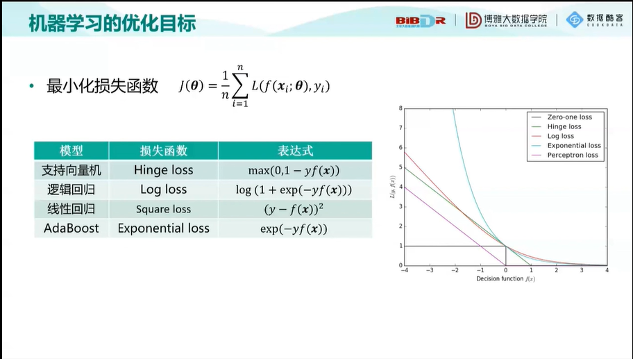
机器学习的优化目标
batch和mini-batch梯度下降

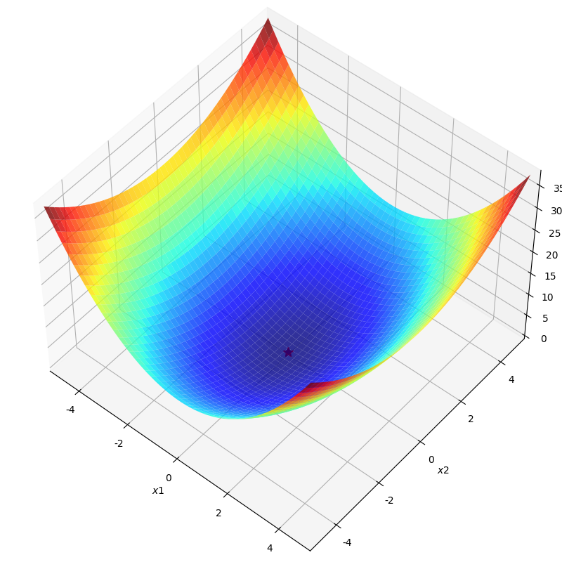
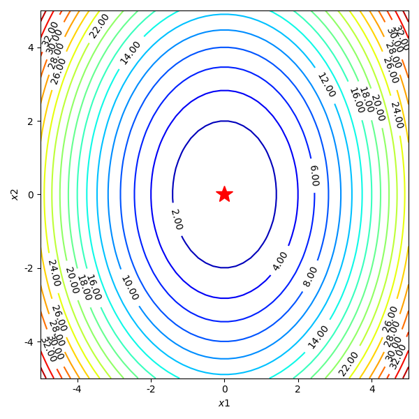
机器学习中常用优化算法的 Python 实践
import matplotlib.pyplot as plt
import numpy as np

from mpl_toolkits.mplot3d import Axes3D
from matplotlib import animation

from autograd import elementwise_grad, value_and_grad,grad
from scipy.optimize import minimize
from scipy import optimize
from collections import defaultdict
from itertools import zip_longest
plt.rcParams['axes.unicode_minus']=False  # 用来正常显示负号
f1 = lambda x1,x2 : x1**2 + 0.5*x2**2 #函数定义
f1_grad = value_and_grad(lambda args : f1(*args)) #函数梯度
def gradient_descent(func, func_grad, x0, learning_rate=0.1, max_iteration=20):
    path_list = [x0]
    best_x = x0
    step = 0
    while step < max_iteration:
        update = -learning_rate * np.array(func_grad(best_x)[1])
        if(np.linalg.norm(update) < 1e-4):
            break
        best_x = best_x + update
        path_list.append(best_x)
        step = step + 1
    return best_x, np.array(path_list)
best_x_gd, path_list_gd = gradient_descent(f1,f1_grad,[-4.0,4.0],0.1,30)
x1,x2 = np.meshgrid(np.linspace(-5.0,5.0,50), np.linspace(-5.0,5.0,50))
z = f1(x1,x2 )
minima = np.array([0, 0]) #对于函数f1,我们已知最小点为(0,0)
fig = plt.figure(figsize=(8, 8))
ax = plt.axes(projection='3d', elev=50, azim=-50)

ax.plot_surface(x1,x2, z, alpha=.8, cmap=plt.cm.jet)
ax.plot([minima[0]],[minima[1]],[f1(*minima)], 'r*', markersize=10)

ax.set_xlabel('$x1$')
ax.set_ylabel('$x2$')
ax.set_zlabel('$f$')

ax.set_xlim((-5, 5))
ax.set_ylim((-5, 5))

plt.show()
dz_dx1 = elementwise_grad(f1, argnum=0)(x1, x2)
dz_dx2 = elementwise_grad(f1, argnum=1)(x1, x2)
fig, ax = plt.subplots(figsize=(6, 6))

contour = ax.contour(x1, x2, z,levels=20,cmap=plt.cm.jet)
ax.clabel(contour,fontsize=10,colors='k',fmt='%.2f')
ax.plot(*minima, 'r*', markersize=18)

ax.set_xlabel('$x1$')
ax.set_ylabel('$x2$')

ax.set_xlim((-5, 5))
ax.set_ylim((-5, 5))

plt.show()