test.csv数据集
,Education,Income
1,10.000000 ,26.658839
2,10.401338 ,27.306435
3,10.842809 ,22.132410
4,11.244147 ,21.169841
5,11.645449 ,15.192634
6,12.086957 ,26.398951
7,12.048829 ,17.435307
8,12.889632 ,25.507885
9,13.290970 ,36.884595
10,13.732441 ,39.666109
11,14.133779 ,34.396281
12,14.635117 ,41.497994
13,14.978589 ,44.981575
14,15.377926 ,47.039595
15,15.779264 ,48.252578
16,16.220736 ,57.034251
17,16.622074 ,51.490919
18,17.023411 ,51.336621
19,17.464883 ,57.681998
20,17.866221 ,68.553714
21,18.267559 ,64.310925
22,18.709030 ,68.959009
23,19.110368 ,74.614639
24,19.511706 ,71.867195
25,19.913043 ,76.098135
26,20.354515 ,75.775216
27,20.755853 ,72.486055
28,21.167191 ,77.355021
29,21.598662 ,72.118790
30,22.000000 ,80.260571
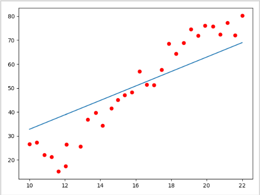
源代码:
import tensorflow as tf
import pandas as pd
import numpy as np
import matplotlib.pyplot as plt
data = pd.read_csv("../data/test.csv")
x = data.Education
y = data.Income
W = tf.Variable(np.random.randn(),name="weight")
b = tf.Variable(np.random.randn(),name="bias")

model = tf.keras.Sequential()
model.add(tf.keras.layers.Dense(1,input_shape=(1,)))
model.compile(optimizer='adam',loss='mse')
history = model.fit(x,y,epochs=5000)
plt.scatter(x,y,c='r')
plt.plot(x,model.predict(x))
plt.show()