本案例采用的是MNIST数据集[1],是一个入门级的计算机视觉数据集。
MNIST数据集已经被嵌入到TensorFlow中,可以直接下载和安装。
1 from tensorflow.examples.tutorials.mnist import input_data
2 mnist=input_data.read_data_sets("MNIST_data/",one_hot=True)
此时,文件名为MNIST_data的数据集就下载下来了,其中one_hot=True为将样本标签转化为one_hot编码。
接下来将MNIST的信息打印出来。
3 print('输入数据:',mnist.train.images)
4 print('输入数据的尺寸:',mnist.train.images.shape)
5 import pylab
6 im=mnist.train.images[0]  #第一张图片
7 im=im.reshape(-1,28)
8 pylab.imshow(im)
9 pylab.show()
输出为:
输入数据: [[0. 0. 0. ... 0. 0. 0.]
 [0. 0. 0. ... 0. 0. 0.]
 [0. 0. 0. ... 0. 0. 0.]
 ...
 [0. 0. 0. ... 0. 0. 0.]
 [0. 0. 0. ... 0. 0. 0.]
 [0. 0. 0. ... 0. 0. 0.]]
输入数据的尺寸: (55000, 784)
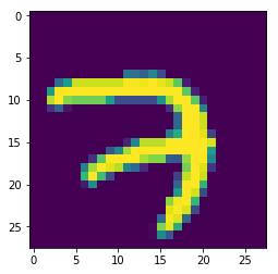
MNIST的图片尺寸为28*28,数据集的存储把所有的图片存在一个矩阵中,将一张图片铺开存为一个行向量,从输出信息我们可以知道训练集包含55000张图片。
MNIST中还包括测试集和验证集,大小分别为10000和5000。
10 print("测试集大小:",mnist.test.images.shape)
11 print("验证集大小:",mnist.validation.images.shape)
测试集用于训练过程中评估模型的准确度,验证集用于最终评估模型的准确度。
接下来就可以进行识别了,采用最简单的单层神经网络的方法,大致顺序就是定义输入-学习参数-学习参数和输入计算-计算损失-定义优化函数-迭代优化
 1 import tensorflow as tf
 2 tf.reset_default_graph()   #清除默认图形堆栈并重置全局默认图形
 3 #定义占位符
 4 x=tf.placeholder(tf.float32,[None,784])   #图像28*28=784
 5 y=tf.placeholder(tf.float32,[None,10])    #标签10类
 6 #定义学习参数
 7 w=tf.Variable(tf.random_normal([784,10])) #权值,初始化为正太随机值
 8 b=tf.Variable(tf.zeros([10]))             #偏置,初始化为0
 9 #定义输出
10 pred=tf.nn.softmax(tf.matmul(x,w)+b)      #相当于单层神经网络,激活函数为softmax
11 #损失函数
12 cost=tf.reduce_mean(-tf.reduce_sum(y*tf.log(pred),reduction_indices=1))  #reduction_indices指定计算维度
13 #优化函数
14 optimizer=tf.train.GradientDescentOptimizer(0.01).minimize(cost)
15 #定义训练参数
16 training_epochs=25   #训练次数
17 batch_size=100       #每次训练图像数量
18 display_step=1       #打印训练信息周期
19 #保存模型
20 saver=tf.train.Saver()
21 model_path="log/521model.ckpt"
22 #开始训练
23 with tf.Session() as sess :
24     sess.run(tf.global_variables_initializer())   #初始化所有参数
25     for epoch in range(training_epochs) :
26         avg_cost=0.                               #平均损失
27         total_batch=int(mnist.train.num_examples/batch_size)   #计算总的训练批次
28         for i in range(total_batch) :
29             batch_xs, batch_ys=mnist.train.next_batch(batch_size)  #抽取数据
30             _, c=sess.run([optimizer,cost], feed_dict={x:batch_xs, y:batch_ys})  #运行
31             avg_cost+=c/total_batch
32         if (epoch+1) % display_step == 0 :
33             print("Epoch:",'%04d'%(epoch+1),"cost=","{:.9f}".format(avg_cost))
34     print("Finished!")
35     #测试集测试准确度
36     correct_prediction=tf.equal(tf.argmax(pred,1),tf.argmax(y,1))
37     accuracy=tf.reduce_mean(tf.cast(correct_prediction,tf.float32))
38     print("Accuracy:",accuracy.eval({x:mnist.test.images,y:mnist.test.labels}))
39     #保存模型
40     save_path=saver.save(sess,model_path)
41     print("Model saved in file: %s" % save_path)
运行得到的结果:
Epoch: 0001 cost= 7.973125283
...
Epoch: 0025 cost= 0.898346810
Finished!
可以看出,损失降低了很多,得到的结果还不错,这只是简单的模型,使用复杂的模型可以得到更好的结果,将在以后给出。
读取保存的模型,测试模型。
 1 print("Starting 2nd session...")
 2 with tf.Session() as sess :
 3     sess.run(tf.global_variables_initializer())
 4     #恢复模型及参数
 5     saver.restore(sess,model_path)
 6
 7     #测试
 8     correct_prediction=tf.equal(tf.argmax(pred,1),tf.arg_max(y,1))
 9     #计算准确度
10     accuracy=tf.reduce_mean(tf.cast(correct_prediction,tf.float32))
11     print("Accuracy: ",accuracy.eval({x:mnist.test.images,y:mnist.test.labels}))
12     #计算输出
13     output=tf.argmax(pred,1)
14     batch_xs,batch_yx=mnist.train.next_batch(2)
15     outputval,predv=sess.run([output,pred],feed_dict={x:batch_xs})
16     print(outputval,predv,batch_ys)
17     #显示图片1
18     im=batch_xs[0]
19     im=im.reshape(-1,28)
20     pylab.imshow(im)
21     pylab.show()
22     #显示图片2
23     im=batch_xs[1]
24     im=im.reshape(-1,28)
25     pylab.imshow(im)
26     pylab.show()