直方图
- 数值型数据可视化的一种方式。
- 如果原始数值型数据经过类别化(分组)处理,则可以使用直方图来观察数据的分布。
- 如果原始数据没有经过分组处理,则使用茎叶图、箱线图、小提琴图、点图、核密度图等来观察数据的分布。
作用:展示数据分布的一种常用方式,通过直方图可观察数据分布的大致形状,能看分布是否对称、快速判断数据是否近似服从正态分布。
import matplotlib.pyplot as plt
plt.rcParams["font.sans-serif"] = ["SimHei"]
plt.rcParams["axes.unicode_minus"] = False
下面来看plt.hist()的语法:
plt.hist(x, bins=None, range=None, normed=False, weights=None, cumulative=False, bottom=None, histtype='bar',
align='mid', orientation='vertical', rwidth=None, log=False, color=None, label=None, stacked=False,
hold=None, data=None, **kwargs)
  Parameters
----------
x : (n,) array or sequence of (n,) arrays  指定要绘制直方图的数据
    Input values, this takes either a single array or a sequency of
    arrays which are not required to be of the same length

bins : integer or array_like or 'auto', optional    指定直方图条形的个数,一种是给定整数,指定绘制多少个条形;一种是给出一个序列,可随意指定间距
    If an integer is given, `bins + 1` bin edges are returned,
    consistently with :func:`numpy.histogram` for numpy version >=
    1.3.

    Unequally spaced bins are supported if `bins` is a sequence.

    If Numpy 1.11 is installed, may also be ``'auto'``.

    Default is taken from the rcParam ``hist.bins``.

range : tuple or None, optional   指定直方图数据的上下界,默认包含绘图数据的max和min
    The lower and upper range of the bins. Lower and upper outliers
    are ignored. If not provided, `range` is (x.min(), x.max()). Range
    has no effect if `bins` is a sequence.

    If `bins` is a sequence or `range` is specified, autoscaling
    is based on the specified bin range instead of the
    range of x.

    Default is ``None``

normed : boolean, optional   是否将直方图的频数转换成频率
    If `True`, the first element of the return tuple will
    be the counts normalized to form a probability density, i.e.,
    ``n/(len(x)`dbin)``, i.e., the integral of the histogram will sum
    to 1. If *stacked* is also *True*, the sum of the histograms is
    normalized to 1.

    Default is ``False``     默认是False,频数图;频率图需要改成True

weights : (n, ) array_like or None, optional  该参数可为每一个数据设置权重
    An array of weights, of the same shape as `x`.  Each value in `x`
    only contributes its associated weight towards the bin count
    (instead of 1).  If `normed` is True, the weights are normalized,
    so that the integral of the density over the range remains 1.

    Default is ``None``

cumulative : boolean, optional   是否需要计算累计频数或频率
    If `True`, then a histogram is computed where each bin gives the
    counts in that bin plus all bins for smaller values. The last bin
    gives the total number of datapoints.  If `normed` is also `True`
    then the histogram is normalized such that the last bin equals 1.
    If `cumulative` evaluates to less than 0 (e.g., -1), the direction
    of accumulation is reversed.  In this case, if `normed` is also
    `True`, then the histogram is normalized such that the first bin
    equals 1.

    Default is ``False``  默认是False,普通的频数或频率图;True,即设置为累计频数图or累计频率图

bottom : array_like, scalar, or None    可以为直方图的每个条形添加基准线,默认0
    Location of the bottom baseline of each bin.  If a scalar,
    the base line for each bin is shifted by the same amount.
    If an array, each bin is shifted independently and the length
    of bottom must match the number of bins.  If None, defaults to 0.

    Default is ``None``

histtype : {'bar', 'barstacked', 'step',  'stepfilled'}, optional   指定直方图的类型,默认为bar,还有barstacked,step,stepfilled
    The type of histogram to draw.

    - 'bar' is a traditional bar-type histogram.  If multiple data
      are given the bars are aranged side by side.

    - 'barstacked' is a bar-type histogram where multiple
      data are stacked on top of each other.

    - 'step' generates a lineplot that is by default
      unfilled.

    - 'stepfilled' generates a lineplot that is by default
      filled.

    Default is 'bar'

align : {'left', 'mid', 'right'}, optional   设置条形边界值的对齐方式,默认mid,还有left and right
    Controls how the histogram is plotted.

        - 'left': bars are centered on the left bin edges.

        - 'mid': bars are centered between the bin edges.

        - 'right': bars are centered on the right bin edges.

    Default is 'mid'

orientation : {'horizontal', 'vertical'}, optional     设置直方图的摆放方向,默认为垂直方向
    If 'horizontal', `~matplotlib.pyplot.barh` will be used for
    bar-type histograms and the *bottom* kwarg will be the left edges.

rwidth : scalar or None, optional   设置直方图条形宽的的百分比
    The relative width of the bars as a fraction of the bin width.  If
    `None`, automatically compute the width.

    Ignored if `histtype` is 'step' or 'stepfilled'.

    Default is ``None``

log : boolean, optional  对数据是否进行log变换
    If `True`, the histogram axis will be set to a log scale. If `log`
    is `True` and `x` is a 1D array, empty bins will be filtered out
    and only the non-empty (`n`, `bins`, `patches`) will be returned.

    Default is ``False``

color : color or array_like of colors or None, optional   直方图的填充色
    Color spec or sequence of color specs, one per dataset.  Default
    (`None`) uses the standard line color sequence.

    Default is ``None``

label : string or None, optional  直方图的标签,可通过legend展示其图例
    String, or sequence of strings to match multiple datasets.  Bar
    charts yield multiple patches per dataset, but only the first gets
    the label, so that the legend command will work as expected.

    default is ``None``

stacked : boolean, optional 当有多个数据时,是否需要将直方图堆叠摆放,默认水平摆放
    If `True`, multiple data are stacked on top of each other If
    `False` multiple data are aranged side by side if histtype is
    'bar' or on top of each other if histtype is 'step'

    Default is ``False``

 facecolor: 直方图颜色
 alpha: 条形透明度
借用Titanic的年龄数据来做例子:
import pandas as pd
data = pd.read_csv(r"G:KaggleTitanic	rain.csv")
data.Age.isnull().sum()
177
存在177个缺失值,我们选择删除掉这些样本。
data.dropna(subset=["Age"], inplace=True)
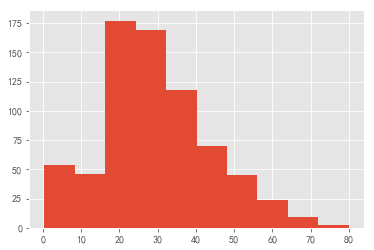
plt.hist(data.Age)  #普通版
plt.show()

下面逐步美化一下
plt.style.use("ggplot")
plt.hist(data.Age, bins=20, color="#FF7373" )
plt.show()

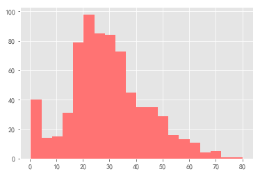
界限不清晰,再加一个边界颜色看看效果。下面先画一个指定组数的,一个指定组距的直方图,根据需要使用。
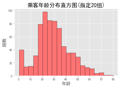
plt.hist(data.Age, bins=20, color="#FF7373",  edgecolor="K")
plt.title("乘客年龄分布直方图(指定20组)", fontsize=18)
plt.xlabel("年龄", size=15)
plt.ylabel("频数", size=15)
plt.show()

plt.hist(data.Age, bins=np.arange(data.Age.min(),data.Age.max(),5), color="#FF7373",  edgecolor="K")
plt.title("乘客年龄直方图(指定组距为5)",fontsize=18)
plt.xlabel("年龄", size=15)
plt.ylabel("频数", size=15)
plt.show()

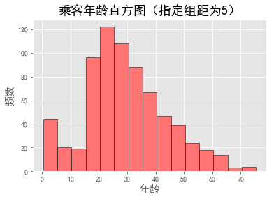
看到年龄分布有点接近正态分布
下面绘制个累计频率直方图
import numpy as np
plt.figure(figsize=(5,6))
plt.hist(data.Age, bins=np.arange(data.Age.min(),data.Age.max(),5), normed=True, cumulative=True, color="#FF7373",  edgecolor="K")
plt.title("乘客年龄累计频率直方图",fontsize=18)
plt.xlabel("年龄", size=15)
plt.ylabel("频数", size=15)
plt.show()


从上图看出乘客年龄的分布情况,接近70%的乘客年龄在35岁以下,接近80%的乘客年龄在40岁以下。
下面给直方图添加两条曲线:正态分布曲线and核密度曲线。一般我们用核密度曲线,正态分布曲线与现实一般都是不一样的,只是理论上的曲线。
import matplotlib.mlab as mlab
plt.figure(figsize=(5.5,5.5))
plt.hist(data.Age, bins = np.arange(data.Age.min(),data.Age.max(), 5), normed = True, color="#FF7373", edgecolor = "k")#画出原数据的频率直方图
x1 = np.linspace(data.Age.min(), data.Age.max(), 1000)    #生成正态分布的数据
normal = mlab.normpdf(x1, data.Age.mean(), data.Age.std())
line1, = plt.plot(x1,normal, "b--", linewidth = 3)        #画出正态分布曲线
kde = mlab.GaussianKDE(data.Age)    #生存核密度数据
x2 = np.linspace(data.Age.min(), data.Age.max(), 1000)
line2, = plt.plot(x2,kde(x2), "g-", linewidth = 3, alpha=0.6)     #画出核密度曲线
plt.legend([line1, line2],[ "正态分布曲线", "核密度曲线"],loc= "best")  #生成图例
plt.title("乘客年龄分布直方图", fontsize=18)
plt.xlabel("年龄", size=15)
plt.ylabel("频率", size=15)
plt.show()

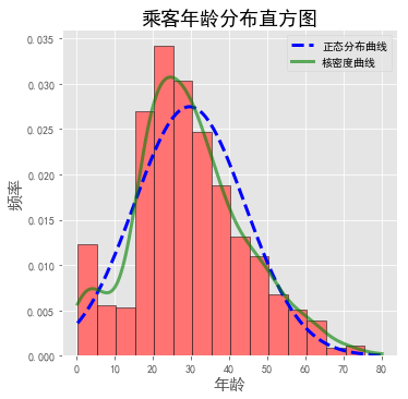
乘客的年龄不服从正态分布,从核密度曲线看出年龄的实际分布情况。