情感分析:基于卷积神经网络
Sentiment Analysis: Using Convolutional Neural Networks
探讨了如何用二维卷积神经网络来处理二维图像数据。在以往的语言模型和文本分类任务中,把文本数据看作一个一维的时间序列,自然地,使用递归神经网络来处理这些数据。实际上,也可以将文本看作一维图像,这样就可以使用一维卷积神经网络来捕捉相邻单词之间的关联。如中所述.. _fig_nlp-map-sa-cnn:本节描述了将卷积神经网络应用于情绪分析的突破性方法:textCNN[Kim,2014]。

Fig. 1. This section feeds pretrained GloVe to a CNN-based architecture for sentiment analysis.
首先,导入实验所需的软件包和模块。
from d2l import mxnet as d2l
from mxnet import gluon, init, np, npx
from mxnet.gluon import nn
npx.set_np()
batch_size = 64
train_iter, test_iter, vocab = d2l.load_data_imdb(batch_size)
1. One-Dimensional Convolutional Layer
在介绍模型之前,让先解释一下一维卷积层是如何工作的。像二维卷积层一样,一维卷积层使用一维互相关运算。在一维互相关运算中,卷积窗口从输入数组的最左边开始,在输入数组上从左到右依次滑动。当卷积窗口滑动到某个位置时,将窗口和核数组中的输入子数组乘以元素求和,得到输出数组中相应位置的元素。如图15.3.2所示,输入是宽度为7的一维数组,内核数组的宽度为2。如所见,输出宽度为7−2+1=6。
第一个元素是通过对最左边的输入子数组(宽度为2)和核数组进行逐元素乘法,然后将结果相加得到第一个元素。
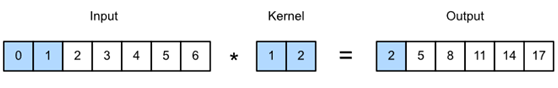
Fig. 2 . One-dimensional cross-correlation operation. The shaded parts are the first output element as well as the input and kernel array elements used in its calculation: 0×1+1×2=20×1+1×2=2。
接下来,在corr1d函数中实现一维互相关。接受输入数组X和内核数组K并输出数组Y。
def corr1d(X, K):
w = K.shape[0]
Y = np.zeros((X.shape[0] - w + 1))
for i in range(Y.shape[0]):
Y[i] = (X[i: i + w] * K).sum()
return Y
现在,将在图2中再现一维互相关运算的结果。
X, K = np.array([0, 1, 2, 3, 4, 5, 6]), np.array([1, 2])
corr1d(X, K)
array([ 2., 5., 8., 11., 14., 17.])
多输入信道的一维互相关运算也类似于多输入信道的二维互相关运算。在每个通道上,对内核及其相应的输入进行一维互相关运算,并将通道的结果相加得到输出。图3显示了具有三个输入信道的一维互相关操作。

Fig. 3 . One-dimensional cross-correlation operation with three input channels. The shaded parts are the first output element as well as the input and kernel array elements used in its calculation: 0×1+1×2+1×3+2×4+2×(−1)+3×(−3)=20×1+1×2+1×3+2×4+2×(−1)+3×(−3)=2。
现在,在图3中再现多输入信道的一维互相关运算的结果。
def corr1d_multi_in(X, K):
# First, we traverse along the 0th dimension (channel dimension) of X and
# K. Then, we add them together by using * to turn the result list into a
# positional argument of the add_n function
return sum(corr1d(x, k) for x, k in zip(X, K))
X = np.array([[0, 1, 2, 3, 4, 5, 6],
[1, 2, 3, 4, 5, 6, 7],
[2, 3, 4, 5, 6, 7, 8]])
K = np.array([[1, 2], [3, 4], [-1, -3]])
corr1d_multi_in(X, K)
array([ 2., 8., 14., 20., 26., 32.])
二维互相关运算的定义告诉,具有多个输入信道的一维互相关运算可以看作是具有单个输入信道的二维互相关运算。如图4所示,也可以将图3中的多个输入信道的一维互相关操作表示为与单个输入信道等效的二维互相关操作。这里,内核的高度等于输入的高度。

Fig. 4. Two-dimensional cross-correlation operation with a single input channel. The highlighted parts are the first output element and the input and kernel array elements used in its calculation: 2×(−1)+3×(−3)+1×3+2×4+0×1+1×2=22×(−1)+3×(−3)+1×3+2×4+0×1+1×2=2。
图2和图3中的输出只有一个信道。如何在二维卷积层中指定多个输出信道。也可以在一维卷积层中指定多个输出通道来扩展卷积层中的模型参数。
2. Max-Over-Time Pooling Layer
有一个一维池化层。TextCNN中使用的max over time pooling层实际上对应于一维全局最大池层。假设输入包含多个通道,并且每个通道由不同时间步上的值组成,则每个通道的输出将是通道中所有时间步的最大值。因此,max over time pooling层的输入在每个通道上可以有不同的时间步长。
为了提高计算性能,通常将不同长度的时序实例组合成一个小批量,并在较短的实例末尾添加特殊字符(如0),使批中每个定时示例的长度一致。自然,添加的特殊字符没有内在意义。因为max over time pooling层的主要目的是捕获最重要的计时特性,通常允许模型不受手动添加字符的影响。
3. The TextCNN Model
TextCNN主要使用一维卷积层和max随时间池层。假设输入文本序列包括n个词汇,d维度词向量。那么输入示例的宽度为n,高度为1,以及d输入通道。
textCNN的计算主要分为以下几个步骤:
定义多个一维卷积核,并使用对输入执行卷积计算。不同宽度的卷积核可以捕获不同数目相邻词之间的相关性。
对所有输出通道执行最大时间池,然后将这些通道的池输出值连接到一个向量中。
连接后的向量通过全连通层转换为每个类别的输出。在这个步骤中可以使用一个脱落dropout层来处理过度拟合。
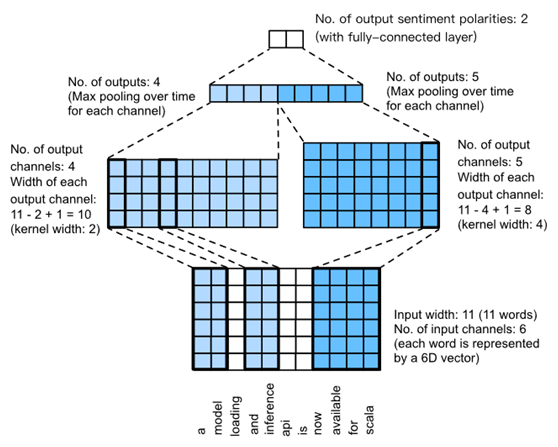
Fig. 5. TextCNN design.
图5给出了一个示例来说明textCNN。这里的输入是一个有11个单词的句子,每个单词由一个6维的单词向量表示。因此,输入序列具有11个和6个输入信道的宽度。假设存在两个宽度分别为2和4的一维卷积核,以及4个和5个输出通道。因此,经过一维卷积计算,四个输出通道的宽度为11−2+1=10,而其五个通道的宽度是11−4+1=8。即使每个通道的宽度不同,仍然可以对每个通道执行max over time pooling,并将9个通道的池输出连接成一个9维向量。最后,使用一个完全连通的层将9维向量转换为二维输出:积极情绪和消极情绪预测。
接下来,将实现textCNN模型。与前一节相比,除了用一维卷积层代替递归神经网络外,这里使用了两个嵌入层,一个具有固定权重,另一个参与训练。
class TextCNN(nn.Block):
def __init__(self, vocab_size, embed_size, kernel_sizes, num_channels,
**kwargs):
super(TextCNN, self).__init__(**kwargs)
self.embedding = nn.Embedding(vocab_size, embed_size)
# The embedding layer does not participate in training
self.constant_embedding = nn.Embedding(vocab_size, embed_size)
self.dropout = nn.Dropout(0.5)
self.decoder = nn.Dense(2)
# The max-over-time pooling layer has no weight, so it can share an
# instance
self.pool = nn.GlobalMaxPool1D()
# Create multiple one-dimensional convolutional layers
self.convs = nn.Sequential()
for c, k in zip(num_channels, kernel_sizes):
self.convs.add(nn.Conv1D(c, k, activation='relu'))
def forward(self, inputs):
# Concatenate the output of two embedding layers with shape of
# (batch size, number of words, word vector dimension) by word vector
embeddings = np.concatenate((
self.embedding(inputs), self.constant_embedding(inputs)), axis=2)
# According to the input format required by Conv1D, the word vector
# dimension, that is, the channel dimension of the one-dimensional
# convolutional layer, is transformed into the previous dimension
embeddings = embeddings.transpose(0, 2, 1)
# For each one-dimensional convolutional layer, after max-over-time
# pooling, an ndarray with the shape of (batch size, channel size, 1)
# can be obtained. Use the flatten function to remove the last
# dimension and then concatenate on the channel dimension
encoding = np.concatenate([
np.squeeze(self.pool(conv(embeddings)), axis=-1)
for conv in self.convs], axis=1)
# After applying the dropout method, use a fully connected layer to
# obtain the output
outputs = self.decoder(self.dropout(encoding))
return outputs
创建一个TextCNN实例。有3个卷积层,内核宽度为3、4和5,全部有100个输出通道。
embed_size, kernel_sizes, nums_channels = 100, [3, 4, 5], [100, 100, 100]
ctx = d2l.try_all_gpus()
net = TextCNN(len(vocab), embed_size, kernel_sizes, nums_channels)
net.initialize(init.Xavier(), ctx=ctx)
3.1. Load Pre-trained Word Vectors
如前所述,加载预先训练的100维手套词向量,初始化嵌入层嵌入和常量嵌入。在这里,前者参加训练,后者有固定的权重。
glove_embedding = d2l.TokenEmbedding('glove.6b.100d')
embeds = glove_embedding[vocab.idx_to_token]
net.embedding.weight.set_data(embeds)
net.constant_embedding.weight.set_data(embeds)
net.constant_embedding.collect_params().setattr('grad_req', 'null')
3.2. Train and Evaluate the Model
现在可以训练模型了。
lr, num_epochs = 0.001, 5
trainer = gluon.Trainer(net.collect_params(), 'adam', {'learning_rate': lr})
loss = gluon.loss.SoftmaxCrossEntropyLoss()
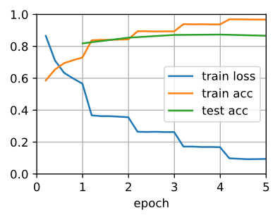
d2l.train_ch13(net, train_iter, test_iter, loss, trainer, num_epochs, ctx)
loss 0.094, train acc 0.968, test acc 0.866
3834.5 examples/sec on [gpu(0), gpu(1)]
下面,使用训练过的模型对两个简单句子的情感进行分类。
d2l.predict_sentiment(net, vocab, 'this movie is so great')
'positive'
d2l.predict_sentiment(net, vocab, 'this movie is so bad')
'negative'
4. Summary
· We can use one-dimensional convolution to process and analyze timing data.
· A one-dimensional cross-correlation operation with multiple input channels can be regarded as a two-dimensional cross-correlation operation with a single input channel.
· The input of the max-over-time pooling layer can have different numbers of timesteps on each channel.
· TextCNN mainly uses a one-dimensional convolutional layer and max-over-time pooling layer.