生成性对抗网络技术实现
Generative Adversarial Networks
以某种形式,使用深度神经网络学习从数据点到标签的映射。这种学习被称为区别性学习,因为希望能够区分猫和狗的照片。量词和回归词都是区别学习的例子。而由反向传播训练的神经网络颠覆了认为在大型复杂数据集上进行区分学习的一切。在仅仅5-6年的时间里,高分辨率图像的分类精度已经从无用的提高到了人类的水平(有一些警告)。将为提供另一个关于所有其区分性任务的细节,在这些任务中,深层神经网络做得非常好。
但是机器学习不仅仅是解决有区别的任务。例如,给定一个没有任何标签的大型数据集,可能需要学习一个简洁地捕捉这些数据特征的模型。给定这样一个模型,就可以抽取与训练数据分布相似的合成数据点。例如,给定大量的人脸照片,可能希望能够生成一个新的照片级真实感图像,看起来似乎似乎来自同一个数据集。这种学习被称为生成性建模。
直到最近,还没有一种方法可以合成新的真实感图像。但是,深度神经网络在区分学习中的成功开辟了新的可能性。在过去三年中,一个大趋势是应用有区别的深层网络来克服通常不认为是有监督学习问题的问题的挑战。递归神经网络语言模型是一个使用判别网络(训练以预测下一个字符)的一个例子,一旦训练,就可以作为一个生成模型。
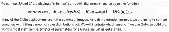
2014年,一篇突破性的论文介绍了生成性对抗性网络(GAN)[Goodfello等人,2014],这是一种巧妙的新方法,可以利用区分模型的能力来获得良好的生成模型。GANs的核心思想是,如果不能区分假数据和真实数据,那么数据生成器是好的。在统计学中,这被称为两个样本测试-一个用来回答是否有数据集的测试
X={x1,…,xn} and X′={x′1,…,x′n}
来自同一分布。大多数统计论文与GAN的主要区别在于后者以建设性的方式运用了这一观点。换句话说,不只是训练一个模型说“嘿,这两个数据集看起来不像来自同一个分布”,而是使用两个样本测试为生成模型提供训练信号。这允许改进数据生成器,直到生成与实际数据相似的内容。至少,需要愚弄分类器。即使分类器是最先进的深层神经网络。

Fig. 1 Generative Adversarial Networks
GAN架构如图1所示。正如所看到的,在GAN架构中有两个部分-首先,需要一个设备(比如说,一个深度网络,但实际上可以是任何东西,比如游戏渲染引擎),可能有可能生成看起来像真实的数据。如果要处理图像,就需要生成图像。如果在处理语音,需要生成音频序列,等等。称之为发启generator网络。第二部分是鉴别器网络。试图区分假数据和真数据。这两个网络互相竞争。生成器网络试图欺骗鉴别器discriminator网络。此时,鉴别器discriminator网络适应新的假数据。这些信息,反过来又被用来改进generator网络,等等。

%matplotlib inline
from d2l import mxnet as d2l
from mxnet import autograd, gluon, init, np, npx
from mxnet.gluon import nn
npx.set_np()
1. Generate some “real” data
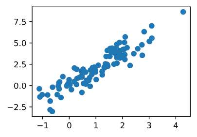
由于这将是世界上最蹩脚的例子,只需从高斯函数中生成数据。
X = np.random.normal(size=(1000, 2))
A = np.array([[1, 2], [-0.1, 0.5]])
b = np.array([1, 2])
data = X.dot(A) + b
让看看得到了什么。这应该是高斯位移,平均值b,以某种相当任意的方式平均协方差矩阵ATA。
d2l.set_figsize((3.5, 2.5))
d2l.plt.scatter(data[:100, 0].asnumpy(), data[:100, 1].asnumpy());
print("The covariance matrix is %s" % np.dot(A.T, A))
The covariance matrix is
[[1.01 1.95]
[1.95 4.25]]
batch_size = 8
data_iter = d2l.load_array((data,), batch_size)
2. Generator
发启Generator网络将是最简单的网络-单层线性模型。这是因为将用高斯数据Generator驱动线性网络。因此,实际上只需要学习参数就可以完美地伪造东西。
net_G = nn.Sequential()
net_G.add(nn.Dense(2))
3. Discriminator
对于鉴别器Discriminator,将更具鉴别力:将使用一个3层的MLP使事情变得更有趣。
net_D = nn.Sequential()
net_D.add(nn.Dense(5, activation='tanh'),
nn.Dense(3, activation='tanh'),
nn.Dense(1))
4. Training
首先定义了一个函数来更新鉴别器discriminator。
#@save
def update_D(X, Z, net_D, net_G, loss, trainer_D):
"""Update discriminator."""
batch_size = X.shape[0]
ones = np.ones((batch_size,), ctx=X.ctx)
zeros = np.zeros((batch_size,), ctx=X.ctx)
with autograd.record():
real_Y = net_D(X)
fake_X = net_G(Z)
# Do not need to compute gradient for net_G, detach it from
# computing gradients.
fake_Y = net_D(fake_X.detach())
loss_D = (loss(real_Y, ones) + loss(fake_Y, zeros)) / 2
loss_D.backward()
trainer_D.step(batch_size)
return float(loss_D.sum())
生成器也同样更新。但是从这里的重复使用熵的标签改变了假数据0到 1。
#@save
def update_G(Z, net_D, net_G, loss, trainer_G): # saved in d2l
"""Update generator."""
batch_size = Z.shape[0]
ones = np.ones((batch_size,), ctx=Z.ctx)
with autograd.record():
# We could reuse fake_X from update_D to save computation.
fake_X = net_G(Z)
# Recomputing fake_Y is needed since net_D is changed.
fake_Y = net_D(fake_X)
loss_G = loss(fake_Y, ones)
loss_G.backward()
trainer_G.step(batch_size)
return float(loss_G.sum())
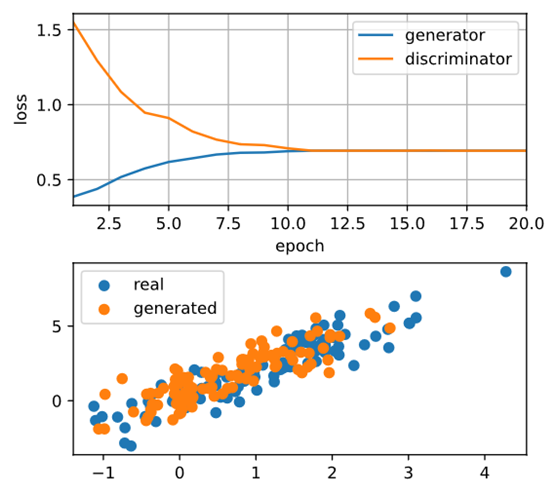
鉴别器Discriminator和产生器Generator都执行带有交叉熵损失的二元逻辑回归。用Adam来平滑训练过程。在每次迭代中,首先更新鉴别器Discriminator,然后更新生成器Generator。将损失和产生的例子都形象化。
def train(net_D, net_G, data_iter, num_epochs, lr_D, lr_G, latent_dim, data):
loss = gluon.loss.SigmoidBCELoss()
net_D.initialize(init=init.Normal(0.02), force_reinit=True)
net_G.initialize(init=init.Normal(0.02), force_reinit=True)
trainer_D = gluon.Trainer(net_D.collect_params(),
'adam', {'learning_rate': lr_D})
trainer_G = gluon.Trainer(net_G.collect_params(),
'adam', {'learning_rate': lr_G})
animator = d2l.Animator(xlabel='epoch', ylabel='loss',
xlim=[1, num_epochs], nrows=2, figsize=(5, 5),
legend=['generator', 'discriminator'])
animator.fig.subplots_adjust(hspace=0.3)
for epoch in range(1, num_epochs+1):
# Train one epoch
timer = d2l.Timer()
metric = d2l.Accumulator(3) # loss_D, loss_G, num_examples
for X in data_iter:
batch_size = X.shape[0]
Z = np.random.normal(0, 1, size=(batch_size, latent_dim))
metric.add(update_D(X, Z, net_D, net_G, loss, trainer_D),
update_G(Z, net_D, net_G, loss, trainer_G),
batch_size)
# Visualize generated examples
Z = np.random.normal(0, 1, size=(100, latent_dim))
fake_X = net_G(Z).asnumpy()
animator.axes[1].cla()
animator.axes[1].scatter(data[:, 0], data[:, 1])
animator.axes[1].scatter(fake_X[:, 0], fake_X[:, 1])
animator.axes[1].legend(['real', 'generated'])
# Show the losses
loss_D, loss_G = metric[0]/metric[2], metric[1]/metric[2]
animator.add(epoch, (loss_D, loss_G))
print('loss_D %.3f, loss_G %.3f, %d examples/sec' % (
loss_D, loss_G, metric[2]/timer.stop()))
现在指定超参数来拟合高斯分布。
lr_D, lr_G, latent_dim, num_epochs = 0.05, 0.005, 2, 20
train(net_D, net_G, data_iter, num_epochs, lr_D, lr_G,
latent_dim, data[:100].asnumpy())
loss_D 0.693, loss_G 0.693, 577 examples/sec
5. Summary
- Generative adversarial networks (GANs) composes of two deep networks, the generator and the discriminator.
- The generator generates the image as much closer to the true image as possible to fool the discriminator, via maximizing the cross-entropy loss, i.e., maxlog(D(x′))maxlog(D(x′)).
- The discriminator tries to distinguish the generated images from the true images, via minimizing the cross-entropy loss, i.e., min−ylogD(x)−(1−y)log(1−D(x))