图像合成与风格转换实战
神经式转移 Neural Style Transfer
如果使用社交分享应用程序或者碰巧是个业余摄影师,对过滤器很熟悉。滤镜可以改变照片的颜色样式,使背景更清晰或人的脸更白。然而,过滤器通常只能改变照片的一个方面。要创建理想的照片,通常需要尝试多种不同的过滤器组合。这个过程就像调整模型的超参数一样复杂。
在本文中,将讨论如何使用卷积神经网络(CNNs)自动将一个图像的样式应用到另一个图像,这一操作称为样式传输。这里,需要两个输入图像,一个内容图像和一个样式图像。使用神经网络来改变内容图像,使其样式与样式图像一致。在图1中,内容图片是作者在西雅图附近的雷尼尔山国家部分拍摄的风景照片。风格意象是一幅秋天橡树油画。输出的复合图像保留了内容图像中对象的整体形状,但应用了风格图像的油画笔触,使整体色彩更加生动。
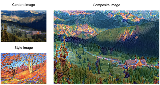
Fig. 1 Content and style input images and composite image produced by style transfer.
1.技术
基于CNN的风格转换模型如图2所示。首先,初始化合成图像。例如,可以将其初始化为内容图像。此合成图像是样式传递过程中唯一需要更新的变量,即样式传递中要更新的模型参数。然后,选取一个预先训练好的CNN进行图像特征提取。这些模型参数在训练期间不需要更新。deepcnn使用多个神经层连续提取图像特征。可以选择某些图层的输出用作内容特征或样式特征。如果使用图2中的结构,预训练的神经网络包含三个卷积层。第二层输出图像内容特征,而第一层和第三层的输出用作样式特征。接下来,使用正向传播(在实线方向)来计算样式传递损失函数,而反向传播(在虚线方向)来更新模型参数,不断更新合成图像。风格转换中使用的损失函数一般有三个部分:
第一,内容丢失用于使合成图像在内容特征方面与内容图像近似。
第二,样式丢失是指通过样式特征使合成图像接近样式图像。
第三. 总变异损失有助于减少合成图像中的噪声。最后,在完成模型训练后,输出风格转换模型参数,得到最终的合成图像。
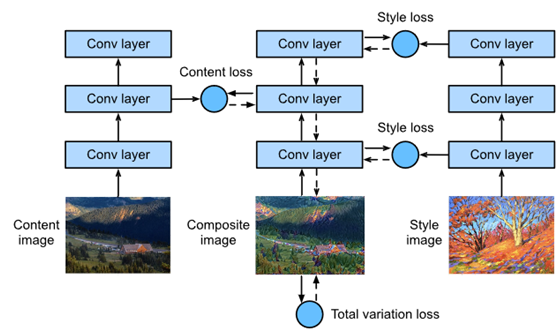
Fig. 2 CNN-based style transfer process. Solid lines show the direction of forward propagation and dotted lines show backward propagation.
接下来,将进行一个实验,帮助更好地理解风格转换的技术细节。
首先,阅读内容和风格图像。通过打印出图像坐标轴,可以看到有不同的尺寸。
%matplotlib inline
from d2l import mxnet as d2l
from mxnet import autograd, gluon, image, init, np, npx
from mxnet.gluon import nn
npx.set_np()
d2l.set_figsize((3.5, 2.5))
content_img = image.imread('../img/rainier.jpg')
d2l.plt.imshow(content_img.asnumpy());

style_img = image.imread('../img/autumn_oak.jpg')
d2l.plt.imshow(style_img.asnumpy());

3. Preprocessing and Postprocessing
下面,定义图像预处理和后处理的函数。预处理功能对输入图像的三个RGB通道中的每一个进行规范化,并将结果转换为可以输入到CNN的格式。后处理函数将输出图像中的像素值恢复为标准化之前的原始值。因为图像打印功能要求每个像素都有一个从0到1的浮点值,所以使用clip函数将小于0或大于1的值分别替换为0或1。
rgb_mean = np.array([0.485, 0.456, 0.406])
rgb_std = np.array([0.229, 0.224, 0.225])
def preprocess(img, image_shape):
img = image.imresize(img, *image_shape)
img = (img.astype('float32') / 255 - rgb_mean) / rgb_std
return np.expand_dims(img.transpose(2, 0, 1), axis=0)
def postprocess(img):
img = img[0].as_in_ctx(rgb_std.ctx)
return (img.transpose(1, 2, 0) * rgb_std + rgb_mean).clip(0, 1)
4. Extracting Features
使用在ImageNet数据集上预先训练的VGG-19模型来提取图像特征。
pretrained_net = gluon.model_zoo.vision.vgg19(pretrained=True)
为了提取图像的内容和风格特征,可以选择VGG网络中某些层的输出。一般来说,输出离输入层越近,提取图像细节信息就越容易。输出越远,提取全局信息就越容易。为了防止合成图像从内容图像中保留太多细节,在输出层附近选择VGG网络层来输出图像的内容特征。这个层叫做内容层。还从VGG网络中选择不同层的输出,以匹配本地和全局样式。这些被称为样式层。VGG网络有五个卷积块。在这个实验中,选择第四个卷积块的最后一个卷积层作为内容层,每个块的第一层作为样式层。可以通过打印预训练后的网络实例来获得这些层的索引。
style_layers, content_layers = [0, 5, 10, 19, 28], [25]
在特征提取过程中,只需要使用从输入层到最接近输出层的内容或样式层的所有VGG层。下面,构建一个新的网络,net,只保留需要使用的VGG网络中的层。然后使用net来提取特征。
net = nn.Sequential()
for i in range(max(content_layers + style_layers) + 1):
net.add(pretrained_net.features[i])
给定输入X,如果只调用前向计算网(X),则只能得到最后一层的输出。因为还需要中间层的输出,所以需要执行逐层计算并保留内容和样式层输出。
def extract_features(X, content_layers, style_layers):
contents = []
styles = []
for i in range(len(net)):
X = net[i](X)
if i in style_layers:
styles.append(X)
if i in content_layers:
contents.append(X)
return contents, styles
接下来,定义了两个函数:get_contents函数获取从内容图像中提取的内容特征,而get_styles函数获取从样式图像中提取的样式特征。由于在训练过程中不需要改变预先训练的VGG模型的参数,所以可以在训练开始前从内容图像中提取内容特征,从样式图像中提取风格特征。由于合成图像是样式转换过程中必须更新的模型参数,因此只能在训练过程中调用extract_features函数来提取合成图像的内容和样式特征。
def get_contents(image_shape, ctx):
content_X = preprocess(content_img, image_shape).copyto(ctx)
contents_Y, _ = extract_features(content_X, content_layers, style_layers)
return content_X, contents_Y
def get_styles(image_shape, ctx):
style_X = preprocess(style_img, image_shape).copyto(ctx)
_, styles_Y = extract_features(style_X, content_layers, style_layers)
return style_X, styles_Y
5. Defining the Loss Function
接下来,将研究用于样式转换的损失函数。损失函数包括内容损失、风格损失和总变化损失。
5.1. Content Loss
与线性回归中使用的损失函数类似,内容丢失使用平方误差函数来测量合成图像和内容图像之间内容特征的差异。平方误差函数的两个输入都是从提取特征extract_features函数获得的内容层输出。
def content_loss(Y_hat, Y):
return np.square(Y_hat - Y).mean()
5.2. Style Loss
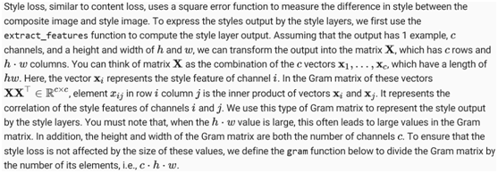
def gram(X):
num_channels, n = X.shape[1], X.size // X.shape[1]
X = X.reshape(num_channels, n)
return np.dot(X, X.T) / (num_channels * n)
自然地,样式丢失的平方误差函数的两个Gram矩阵输入来自合成图像和样式图像样式层输出。这里,假设已经预先计算了样式图像的Gram矩阵。
def style_loss(Y_hat, gram_Y):
return np.square(gram(Y_hat) - gram_Y).mean()
5.3. Total Variance Loss
有时,学习到的合成图像有很多高频噪声,特别是亮像素或暗像素。一种常用的降噪方法是全变差去噪。假设xi,j表示(i,j)坐标处的像素值,因此总方差损失为:

尽量使相邻像素的值尽可能相似。
def tv_loss(Y_hat):
return 0.5 * (np.abs(Y_hat[:, :, 1:, :] - Y_hat[:, :, :-1, :]).mean() +
np.abs(Y_hat[:, :, :, 1:] - Y_hat[:, :, :, :-1]).mean())
5.4. The Loss Function
风格转移的损失函数是内容损失、风格损失和总方差损失的加权和。通过调整这些权重超参数,可以根据保留内容、传输样式和降噪的相对重要性来平衡。
content_weight, style_weight, tv_weight = 1, 1e3, 10
def compute_loss(X, contents_Y_hat, styles_Y_hat, contents_Y, styles_Y_gram):
# Calculate the content, style, and total variance losses respectively
contents_l = [content_loss(Y_hat, Y) * content_weight for Y_hat, Y in zip(
contents_Y_hat, contents_Y)]
styles_l = [style_loss(Y_hat, Y) * style_weight for Y_hat, Y in zip(
styles_Y_hat, styles_Y_gram)]
tv_l = tv_loss(X) * tv_weight
# Add up all the losses
l = sum(styles_l + contents_l + [tv_l])
return contents_l, styles_l, tv_l, l
6. Creating and Initializing the Composite Image
在样式传输中,合成图像是唯一需要更新的变量。因此,可以定义一个简单的模型,生成图像,并将合成图像作为模型参数。在模型中,正向计算只返回模型参数。
class GeneratedImage(nn.Block):
def __init__(self, img_shape, **kwargs):
super(GeneratedImage, self).__init__(**kwargs)
self.weight = self.params.get('weight', shape=img_shape)
def forward(self):
return self.weight.data()
接下来,定义get_inits函数。此函数创建一个复合图像模型实例,并将其初始化为图像X。在训练之前,将计算样式图像的各个样式层的Gram矩阵styles_Y_gram。
def get_inits(X, ctx, lr, styles_Y):
gen_img = GeneratedImage(X.shape)
gen_img.initialize(init.Constant(X), ctx=ctx, force_reinit=True)
trainer = gluon.Trainer(gen_img.collect_params(), 'adam',
{'learning_rate': lr})
styles_Y_gram = [gram(Y) for Y in styles_Y]
return gen_img(), styles_Y_gram,
7. Training
在模型训练过程中,不断提取合成图像的内容和风格特征,并计算损失函数。同步函数如何强制前端等待计算结果。因为只每隔50个时间段调用一次asscalar同步函数,这个过程可能会占用大量内存。因此,在每个时间段期间调用waitall同步函数。
def train(X, contents_Y, styles_Y, ctx, lr, num_epochs, lr_decay_epoch):
X, styles_Y_gram, trainer = get_inits(X, ctx, lr, styles_Y)
animator = d2l.Animator(xlabel='epoch', ylabel='loss',
xlim=[1, num_epochs],
legend=['content', 'style', 'TV'],
ncols=2, figsize=(7, 2.5))
for epoch in range(1, num_epochs+1):
with autograd.record():
contents_Y_hat, styles_Y_hat = extract_features(
X, content_layers, style_layers)
contents_l, styles_l, tv_l, l = compute_loss(
X, contents_Y_hat, styles_Y_hat, contents_Y, styles_Y_gram)
l.backward()
trainer.step(1)
npx.waitall()
if epoch % lr_decay_epoch == 0:
trainer.set_learning_rate(trainer.learning_rate * 0.1)
if epoch % 10 == 0:
animator.axes[1].imshow(postprocess(X).asnumpy())
animator.add(epoch, [float(sum(contents_l)),
float(sum(styles_l)),
float(tv_l)])
return X
接下来,开始训练模型。首先,将内容和样式图像的高度和宽度设置为150×225像素。使用合成图像初始化内容。
ctx, image_shape = d2l.try_gpu(), (225, 150)
net.collect_params().reset_ctx(ctx)
content_X, contents_Y = get_contents(image_shape, ctx)
_, styles_Y = get_styles(image_shape, ctx)
output = train(content_X, contents_Y, styles_Y, ctx, 0.01, 500, 200)
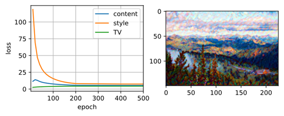
如所见,合成图像保留了内容图像的风景和对象,同时引入了样式图像的颜色。因为图像比较小,细节有点模糊。为了获得更清晰的合成图像,使用更大的图像尺寸训练模型:900×600。将之前使用的图像的高度和宽度增加四倍,并初始化更大的合成图像。
image_shape = (900, 600)
_, content_Y = get_contents(image_shape, ctx)
_, style_Y = get_styles(image_shape, ctx)
X = preprocess(postprocess(output) * 255, image_shape)
output = train(X, content_Y, style_Y, ctx, 0.01, 300, 100)
d2l.plt.imsave('../img/neural-style.png', postprocess(output).asnumpy())

如所见,由于图像尺寸较大,每个纪元花费的时间更长。如图3所示,合成图像因其尺寸较大而保留了更多细节。合成图像不仅有像样式图像那样的大色块,而且这些块甚至具有画笔笔触的微妙纹理。

Fig. 3 900×600900×600 composite image.
8. Summary
- The loss functions used in style transfer generally have three parts: 1. Content loss is used to make the composite image approximate the content image as regards content features. 2. Style loss is used to make the composite image approximate the style image in terms of style features. 3. Total variation loss helps reduce the noise in the composite image.
- We can use a pre-trained CNN to extract image features and minimize the loss function to continuously update the composite image.
- We use a Gram matrix to represent the style output by the style layers.