介绍

目标检测系统总概：（1）输入一张图。（2）提取候选区域（2k左右）。（3）使用CNN计算每个候选区域的特征。（4）使用class-specific linear SVMs来分类。

使用R-CNN作目标检测

R-CNN由三个模块构成：（1）第一个模块产生候选区域。（2）第二个模块是一个大型的CNN网络，用来从候选区域提取固定长度的特征向量。（3）第三个模块是一组class-specific linear SVMs。

模型设计

候选区域

这里作者用到了“选择性搜索”（selective search），主要思路是根据图像的颜色、纹理、尺寸和空间交叠等参数来把图像分成许多子块，这种方法比穷举法效率更高。具体可以看这里：选择性搜索（selective search），Selective Search for Object Detection (C++ / Python)。

下面简单的使用代码实现selective search的算法：

#!/usr/bin/env python
'''
Usage:
    ./ssearch.py input_image (f|q)
    f=fast, q=quality
Use "l" to display less rects, 'm' to display more rects, "q" to quit.
'''
 
import sys
import cv2
 
if __name__ == '__main__':
    # If image path and f/q is not passed as command
    # line arguments, quit and display help message

 
    # speed-up using multithreads
    cv2.setUseOptimized(True);
    cv2.setNumThreads(4);
 
    # read image
    im = cv2.imread("D:\tensorflow\image.jpg")
    # resize image
    newHeight = 200
    newWidth = int(im.shape[1]*200/im.shape[0])
    im = cv2.resize(im, (newWidth, newHeight))    
 
    # create Selective Search Segmentation Object using default parameters
    ss = cv2.ximgproc.segmentation.createSelectiveSearchSegmentation()
 
    # set input image on which we will run segmentation
    ss.setBaseImage(im)
 
    # Switch to fast but low recall Selective Search method
    ss.switchToSelectiveSearchFast()
    # Switch to high recall but slow Selective Search method
    #ss.switchToSelectiveSearchQuality()
    # if argument is neither f nor q print help message
 
    # run selective search segmentation on input image
    rects = ss.process()
    print('Total Number of Region Proposals: {}'.format(len(rects)))
     
    # number of region proposals to show
    numShowRects = 100
    # increment to increase/decrease total number
    # of reason proposals to be shown
    increment = 50
 
    while True:
        # create a copy of original image
        imOut = im.copy()
 
        # itereate over all the region proposals
        for i, rect in enumerate(rects):
            # draw rectangle for region proposal till numShowRects
            if (i < numShowRects):
                x, y, w, h = rect
                cv2.rectangle(imOut, (x, y), (x+w, y+h), (0, 255, 0), 1, cv2.LINE_AA)
            else:
                break
 
        # show output
        cv2.imshow("Output", imOut)
 
        # record key press
        k = cv2.waitKey(0) & 0xFF
 
        # m is pressed
        if k == 109:
            # increase total number of rectangles to show by increment
            numShowRects += increment
        # l is pressed
        elif k == 108 and numShowRects > increment:
            # decrease total number of rectangles to show by increment
            numShowRects -= increment
        # q is pressed
        elif k == 113:
            break
    # close image show window
    cv2.destroyAllWindows()

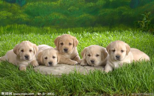
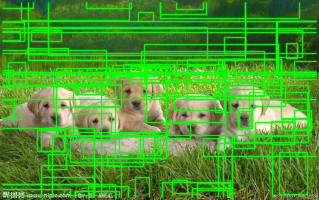
结果如下图：

特征提取

使用Caffe实现的CNN来对每个候选区域进行特征提取，每个区域提取4096维的特征向量。使用包含5个卷积层和2个全连接层的CNN对减去均值的、大小为227*227的RGB图像通过前向传播来计算特征。为了使训练数据与CNN（要求输入数据为固定的227*227）匹配，需要对输入图像进行变形。

注：CNN见以下论文：《A. Krizhevsky, I. Sutskever, and G. Hinton. ImageNet classification with deep convolutional neural networks. In NIPS, 2012.》

非极大值抑制

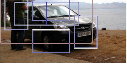
使用selective search的快速模式来提取图像的2000多个候选区域，然后对每个候选区域进行变形，通过前向传播在对应的层得到特征。接着，对每一个类，使用针对该类训练过的SVM计算提取到的特征在该类上的分数。这样便得到了一张图的所有区域的Score，接着作者使用一种称为“非极大值抑制”的方法（每个类都是独立处理的）排除一些区域。如下的图像，关于“car”类会得到很多的方框，分类器根据分值从大到小排序：A,B,C,D,E,F。从最大概率的框A开始，判断B-F与之的重合区域，如果大于一个阈值，则丢弃概框。接着，最框B开始（如果B没有被丢弃的话），重复前面的操作。

训练

有监督的预训练

作者先把CNN在一个辅助数据集“ILSVRC 2012”上做了一个预训练（图像进行了分类标注，但没有边框标注），这应该是迁移学习的思想吧。

微调：fine-tuning

为了使CNN可以适用于目标检测任务，假设要检测的物体类别有N类，那么我们就需要把上面预训练阶段的CNN模型的最后一层给替换掉，替换成N+1个输出的神经元(加1，表示还有一个背景)，然后这一层直接采用参数随机初始化的方法，其它网络层的参数不变；接着就可以开始继续SGD训练了。开始的时候，SGD学习率选择0.001，在每次训练的时候，我们batch size大小选择 128，其中32个是正样本、96个是负样本。

这里提到一个概念：定位精度评价公式（IOU），该公式定义了两个bounding box的重叠度，作者将IOU>0.5的bounding box判定为正，其余判定为负。

目标分类器

通过实验，得到最佳IOU重叠阈值为0.3。分类器输出的区域的IOU大于0.3的判定为正样本，否则判定为负样本。

作者在这里引入了“Hard negative mining”方法，首先是negative，即负样本，其次是hard，说明是困难样本，也就是说在对负样本分类时候，loss比较大（label与prediction相差较大）的那些样本，也可以说是容易将负样本看成正样本的那些样本，例如ROI里没有物体，全是背景，这时候分类器很容易正确分类成背景，这个就叫easy negative；如果ROI里有二分之一个物体，标签仍是负样本，这时候分类器就容易把他看成正样本，这时候就是had negative。hard negative mining就是多找一些hard negative加入负样本集，进行训练，这样会比easy negative组成的负样本集效果更好。主要体现在虚警率更低一些（也就是false positive少）。